Let's formulate profit maximization condition for the monopolist. To do this, we find the derivative of profit (P) with respect to Q and equate it to zero
or MC=MR≠P (7.2)
Let's go back to the numerical example. If with an increase in the volume of production by 1 product, the total costs of the monopolist increase by 250 den. units then his profit increases by (300-250) den. units and the monopolist is interested in expanding production and raising prices. He will do this until his marginal revenue equals his marginal cost. If, on the contrary, MC >MR and are equal, for example, 350 den. unit, the monopolist, seeking to maximize profits, will reduce output and raise prices.
To maximize profit, a firm must achieve a level of output at which marginal revenue equals marginal cost. On the rice. 7.13 market demand curve D is the monopolist's average income curve. The unit price that the monopolist will receive is a function of output.
It also shows marginal revenue curves MR and marginal cost MC. Marginal revenue and marginal cost coincide at output QM . Using the demand curve, we can determine the price P M , which corresponds to a given quantity of products QM . The graph illustrates that when output is higher or lower QM the manufacturer will make less profit because Q1< Q M the loss of profit is associated with the production of too little quantity of products and selling at too high a price (P 1), and with Q 2 > Q M losses are associated with the production of too many products and selling at too low a price (P 2).
So, striving for the maximum profit, the monopoly chooses the volume of production at which MC = MR . The point of intersection of these graphs is indicated by point K, since the point of profit maximization by a monopoly is called the Cournot point. On the pic 7.14 monopoly profit per unit of monopoly output QM equal to the length of the segment FN (P M >AC). The total profit of the monopoly on the entire output is equal to the area P M FNL (on the rice. 7.14 shaded area).
A monopolist usually produces less than perfect competition and at higher prices.
Having a monopoly, however, does not guarantee profit.


Rice. 7.15.Loss-making monopoly
On the chart (Fig. 7.15) there is not enough demand to make a profit at the point where MC = MR , the firm incurs economic losses, since P<АС.
To the content of the book: Prices and pricing
See also:
Let us assume that, as in the models of perfect competition, the goal of a particular monopolist is to maximize economic profit. As before, in this case this means that, in the short run, the monopolist must maintain the level of output at which the difference between gross income and gross costs will be greatest. Such a decision is less forced for a monopolist than for a competing firm, since the monopolist has to expend less effort to survive. In other words, the evolution from competition to monopoly has meant that under monopoly production, profit maximization requires less effort. Later in this chapter, we will consider the alternative assumption that monopolists are more willing to maximize output than economic profit. But for now, we will explore the behavior of a monopolist whose goal is to maximize profits.
Monopoly Gross Profit Curve
The main difference between monopoly and perfect competition is the nature of the change in gross and marginal revenues with changes in production volumes. As we saw in Chapter 11, the demand curve for a perfectly competitive firm is a horizontal line at the short-term equilibrium price P*. A perfectly competitive firm simply accepts the price because its output is too small to have any appreciable effect on the market price. In this case, the gross income curve of a perfect competing firm is a ray emanating from the origin, with a slope equal to P * (Fig. 12.2).
)?
Now suppose that the monopoly firm has a downward-sloping demand curve (Figure 12.3). As for any firm, the gross income of such a monopolist is equal to the product of the price by the number of products. For example, at point L of this demand curve, the monopolist sells 100 units during the week. products at a price of $60 per unit, which would give him a gross income of $6,000 per week. At point B, he will sell 200 units. at a price of $40 per unit and earn a gross income of $8,000 per week, etc. The difference between a monopoly and perfect competition is that a monopolist who wants to sell more products must lower the price, and not only unit of production, but also for all previously released products. As discussed in Chapter 5, the effect of a sloping demand curve is that gross income is not proportional to the amount of output over the entire segment. As in perfect competition, the monopolist's gross income curve (the central part of Figure 12.3) passes through the origin, because in either case, if there were no sales, there would be no income. But with a decrease in price, the gross income of the monopolist does not increase linearly with respect to the volume of output, but reaches a maximum value at the volume of output corresponding to the midpoint on the demand curve (B in the upper part of Fig. 12.3), after which it begins to decline. Relevant values price elasticity demand are shown at the bottom of fig. 12.3. Note that gross income reaches its maximum when the price elasticity of demand is 1.
Price (USD/unit of production)
EXERCISE 12.1
Draw graphically the curve of the monopolist's gross income, for which the demand curve is represented by the equation: Р= 100 - 2().
At the top of Fig. 12.4 the curve of short-term gross costs and a curve of the gross income of the monopolist, corresponding to the curve of demand shown on fig. 12.3. The economic profit shown at the bottom of the figure is positive in the range from Q = 45 to Q - 305 and negative for all other numerical values of Q. The point of maximum profit corresponds to the level of output Q * = 175 units. per week, which is located to the left of the volume of output pro-duktsii, maximizing gross income (Q = 200).
We note from Fig. 12.4 that the vertical distance between the short-term curves of gross costs and gross income is greatest when these curves are parallel, which corresponds to the point Q \u003d 175. Let's assume a different situation - for example, that at the point of profit maximization the curve of gross costs rises more steeply, than the gross income curve. Then it would be possible to save by reducing the volume of production, since the cost reduction in this case would exceed the corresponding reduction in gross income. Conversely, if the gross cost curve were less steep than the gross income curve, this monopolist would be able to make higher profits by increasing output, since gross income would now increase faster than gross costs.?
marginal revenue
The slope of the gross cost curve at any level of output is, by definition, equal to the marginal cost at this level of output. The slope of the gross revenue curve is also, by definition, a marginal revenue of 1. As with a competing firm, we can consider a monopolist's marginal revenue as some amount by which its gross revenue will change when sales volume changes by 1 unit. Assuming that AT(O) represents the change in gross income that occurs in response to some small change in output (AO), then marginal revenue (MN(O)) can be determined from the equation:
Using this definition, an experienced monopolist seeking to maximize profits in the short term will produce output (? *, at which
MC(0*) = MI(0*).2
Recall that a similar condition for a competing firm was to choose a level of production at which price and marginal cost were equal. Note that marginal revenue (MR) and price (P) under perfect competition are the same (when such a firm increases its output by 1 unit, its gross income increases by P). From this we can conclude that the condition of profit maximization by a firm operating in conditions of perfect competition is just a special case of equation (12.2).
For a monopoly firm, marginal revenue will always be less than price. To verify the validity of this statement, consider the demand curve in Fig. 12.5. Suppose that the monopolist plans to increase the volume of production from O0 \u003d 100 to C?0 + L 0~150 units. in Week. The gross income of this monopolist from the sale of 100 units. per week is $ 60 / unit. 100 units/week = $6,000/week In order to sell an additional L O = 50 units/week, he must reduce his price to 60 - AP =
- $50/unit, which means that his new gross income will be $50/unit. 150 units/week = $7,500/week To determine the marginal income, it is enough to subtract the original gross income ($6,000 per week) from the new gross income ($7,500 per week) and divide the resulting difference by
1 In the terminology of computational techniques, marginal revenue is a derivative function 2 This condition can also be confirmed if we take into account that the first condition for maximizing profit is determined by the expression
3 In fact, there is an exception to this statement - for the case of perfect discrimination carried out by a monopolist, which will be discussed later. - Approx. ed.
well, increments in output (AO \u003d 50 units per week). As a result, we get MN(O0 = 100) = ($7,500/week - $6,000/week)/50 units/week. = $30/unit Obviously, this value is less than the original price of $60 per unit.
Consider another useful relationship between marginal revenue and the amount of gain from new sales and losses from sales of previously produced products at a new, lower price. On fig. 12.5 The area of rectangle B ($2,500 per week) represents the gain from additional sales at a reduced price; the area of rectangle A ($1,000 per week) is the loss incurred as a result of the sale of the previously issued 100 units. items per week at 50 instead of $60 per item. Marginal revenue is the difference between the gain from additional sales and the loss from selling at a reduced price, divided by the change in the number of sales. As a result, we get [(2500 dollars / week.
- $1,000/week)/50 units/week] again $30/unit.
R (USD/unit)
Rice. 12.5. Changes in gross income as a result of price reductions The area of rectangle A ($1,000 per week) is the loss incurred as a result of the sale of previously manufactured products at a reduced price; the area of rectangle B ($2,500 per week) is the gain from selling additional items at the new, lower price. Marginal revenue is the difference between the areas of these two rectangles ($2,500/week - $1,000/week = $1,500/week) divided by the change in output (50 units/week). In this case, the ML is $30 per unit, which is less than the new price of $50 per unit.
To investigate changes in marginal revenue as we move along the demand curve, consider a specific linear demand curve (Figure 12.6). Assume that this monopolist plans to increase output from O0 to
O0 + AO units His gross income from the sale of O0 will be P0 (? 0. To sell an additional AO unit, he will have to reduce the price of his products to P0 - AP, while his new gross income will be (P0 - AP) (O0 + AO) , which is equivalent to the expression: PO00 + PyA0 - A P0$ - A PAO To calculate marginal revenue, up to
it is enough to simply subtract the initial gross income P0 () 0 from the new gross income and divide this difference by the value of the change in output D (>. As a result, we get: МЯ (О0) = Р0 - (DR / D0Sho - АР. that MR(O0) is less than P. Since AP tends to 0, the expression for calculating marginal revenue is:
leda>)=l>--^a>(12.h)
Equation 12.3 allows you to intuitively evaluate the result when the output (A O) changes by one unit: then P0 will be the gain from the sale of this additional unit of output, and (D7UL0OO \u003d APb0 will be the loss from the sale of all units of the existing level of production at a reduced price Equation 12.3 also shows that marginal revenue is less than price at all positive levels of production.
Rectangle area B more area rectangle A (Fig. 12.6), which means that the marginal income at the level of output (? 0 is positive. However, with an increase in the level of production, that is, when it goes beyond the midpoint M on the demand curve, marginal income with a further expansion of production output will be negative.For example, the fact that the area of rectangle C is greater than the area of rectangle D means that marginal revenue at output level 01 is less than 0.
USD/unit
Rice. 12.6. Marginal revenue on the demand curve When O is located to the left of the midpoint M on a straight-line demand curve (for example, O = O0), the gain from additional sales (area B) will be greater than the loss from price reduction at the existing level of sales (area A) . When O is located to the right of the midpoint (for example, O = O,), the gain from additional sales (area b) will be less than the loss from price reduction at the existing level of sales (area C). At the midpoint of the demand curve, gains and losses are equal. This means that the marginal revenue at this point is 0.
Marginal revenue and elasticity
At appropriate points on the demand curve, another useful relationship is also true, relating marginal revenue to price elasticity of demand. Recall that in Chapter 5, the price elasticity of demand at the point (O, P) was determined by the following expression:
-
D
Here A() and AP have opposite signs, since the demand curve slopes down. In contrast, in Equation 12.3, AO and AR, also representing changes in P and 0 as they move along the demand curve, are positive. Suppose we redefine the quantities A? and ARiz Equation 12.4 so that they are positive. Then this equation will take the form:
I I A O R
M=dr? * - (12.5)
Now that A0 and AP are both positive, we can relate Equation 12.5 to Equation 12.3. If we now solve equation 12.5 with AP / A () = = P / (OY) and substitute this value in equation 12.3, we get:
Equation 12.6 clearly shows that the lower the price elasticity of demand, the more the price will exceed marginal revenue1. This expression also shows that when price elasticity is infinite, marginal revenue and price are exactly the same. (Recall from Chapter 11 that price and marginal revenue are the same for a competing firm with a horizontal, or perfectly elastic, demand curve.)
Graphical depiction of marginal revenue
Equation 12.6 can be used without special work indicate on the graph the values \u200b\u200bof marginal income corresponding to different points on the demand curve. Consider, for example, a demand curve that looks like a straight line (Fig. 12.7), which intersects the y-axis at the point corresponding to the price value P = 80. At this point, the elasticity of demand is infinitely large. This means that MR(0) = 80(1 - 1/°o) = 80. Although marginal revenue will be less than the price for the monopolist, both these values are exactly the same at 0=0. The reason for this is that at "zero" output, there are no sales at a price reduced to a value that allows for income.
t__chtk__^t=p^p=p (^p) II M-" m
40 s!0 1 Equation 12.6 can be derived using the following transformations:
?
?
Now let's move down, say, 1/4 of the entire length of the demand curve, to point A (100, 60). At this point |r|| \u003d 3 (recall from Chapter 5 that the elasticity of demand at any point located on the demand curve, which looks like a straight line, is simply the ratio of the length of the segment of the demand curve located below this point to the length of the upper segment). Thus, at this point we have ASCHIO) \u003d 60 (1 - 1/3) \u003d 40.
At the point? (200,40), located in the middle of the demand curve, M = 1. Obviously, in this case, ML (200) = 40 (1 - 1/1) = 0. This result confirms the conclusion made earlier (see chapter 5) that gross income is maximum at the midpoint of a straight-line demand curve, in which the elasticity is 1.
Finally, consider point C (300, 20) located on the demand curve at a distance of 3/4 of its Length from the point of intersection with the y-axis. In this case (l! ~ 1/3 and, accordingly, ASch300) = 20 = 20 (-2) = 40. Thus, when R = 300 units, the gross income from the sale of each additional unit of production is reduced by $40.
Carrying out similar calculations at each point of the demand curve, it is easy to see that the marginal revenue curve obtained by appropriately transforming the demand curve is a straight line, the slope of which is 2 times steeper than the slope of the demand curve. The marginal revenue curve crosses the x-axis just below the midpoint of the demand curve, and all values of marginal revenue to the right of this point will be negative. Thus, at all points located to the right of the projection of the midpoint of the demand curve on the x-axis, the absolute value of price elasticity will be less than 1. The fact that the marginal income in this area is negative is in good agreement with the conclusion
As discussed in Chapter 5, a price reduction will reduce gross income in all cases where demand is inelastic with respect to price.
EXAMPLE 12.1
Construct a marginal revenue curve corresponding to the demand curve, which corresponds to the equation P = 1230.
The marginal revenue curve will be twice as steep as the given demand curve. It is obvious that these conditions are uniquely satisfied by only one curve shown in Fig. 12.8 and expressed by the equation МЯ=П-60.
Rice. 12.8. Linear Demand Curve and Corresponding Marginal Revenue Curve The MI marginal revenue curve cuts off the same segment on the vertical axis as the demand curve and has a slope that is twice as steep as the corresponding linear demand curve.
The general formula for a linear demand curve can be written as P = ab(), where a and b are positive numbers. The corresponding marginal revenue curve can be expressed by the equation ML = a2 b0.
EXERCISE 12.2
Draw graphically the demand and marginal revenue curves of a monopolist whose market demand curve has the form P ~ 100 - 2(7.
Graphical interpretation of the profit maximization condition in the short run
Recall that Chapter 11 provides a graphical interpretation of the profit maximization point for a competing firm in the short run. A similar graphical interpretation is also possible for a monopolist. Let's assume that the state of affairs of the monopolist is characterized by the curves of demand, marginal revenue and short-term costs depicted in fig. 12.9. The level of output that maximizes the firm's profit is 0*, and it corresponds to the intersection point of the marginal revenue and marginal cost curves. At this level of output, the monopolist can charge a price /*, which will allow him to earn an economic profit equivalent to the area of the shaded rectangle R.
Rice. 12.9. The price and level of production that maximize the monopolist's profit
The maximum profit is achieved at the volume of production O *, when the gain from an increase in output (or losses from a decrease in output), denoted by MR, is exactly equal to the costs of expanding output (or the savings resulting from a reduction in output products), designated SMC. At O*, the firm charges a price P* and earns economic profit P.
EXAMPLE 12.2
Noah in this example 20. Assuming MH = MS, we obtain the equation 100 - 40 = 20; solving it, it is easy to determine that the level of output that provides the company with maximum profit is O * \u003d 20. Substituting the value of O * \u003d 20 into the analytical expression of the demand curve, we find that the price that provides the company with maximum profit profit is Р* = 60. This solution is graphically depicted in fig. 12.10. In the same place the curve of average gross costs of a monopolist is shown. Note that with O *, the average gross costs (ATC) are equal to 52. This means that each sold unit of production will bring to the monopolist an economic profit equal to 60 - 52 \u003d 8. With the number of sold units of production O * \u003d 20, the total economic profit will be 160.
$/0
Rice. 12.10. Price and level of production that maximize profits at given functions costs and demand
Note that the fixed costs of the considered monopolist (and this is confirmed by the location of the curves in Fig. 12.10) were not taken into account when determining the level of output and prices that maximize profits. Such a conclusion suggests itself intuitively, since fixed costs have nothing to do with either gains or losses due to changes in production volumes.
EXERCISE 12.3
How will the profit-maximizing price and output change if the monopolist's gross cost curve in Example 12.2 is TC ~ 640 + 40 0?
Profit maximizing monopolist does not produce the amount of output corresponding to the inelastic part of the demand curve
A profit maximizing monopolist will never produce a quantity that matches the inelastic portion of the demand curve. In this case, if the monopolist increases the price of its products, its gross income will also increase. At the same time, an increase in prices leads to a reduction in production volume and, as a result, to a decrease in gross production costs. Since economic profit is the difference between gross income and gross costs, it must necessarily increase in response to an increase in price from its initial value on the inelastic part of the demand curve. Therefore, the level of production that maximizes profit must correspond to the elastic part of the demand curve, where a further increase in price will cause a simultaneous decrease in both income and costs.
Profit maximizing markup
The profit maximization condition, according to which MJ - MC, can be combined with the formula 12.6, according to which MJ - R. Solving these 2 equations, we can formulate a pricing rule for a profit-maximizing monopolist:
R-MS 1 --i-! (,2-7>
The left side of Equation 12.7 is the difference between price and marginal cost, expressed as a fraction of the profit-maximizing price. If the price elasticity of demand faced by the monopolist is, for example, 2, then the price increase to a value that ensures maximum profit, will be U2. This means that the profit-maximizing price must be twice the marginal cost. Equation 12.7 shows that the profit-maximizing markup increases more slowly as demand becomes more elastic. In the case of infinitely elastic demand, the profit-maximizing markup is 0 (which means that P is MC), i.e. we arrive at the same result as in the presence of perfect competition.
Conditions under which the monopolist must stop production
In the study of perfect competition, it was shown that it is advantageous for a competing firm to quickly terminate its activity if the price falls below the minimum value of average variable costs. A similar condition for a particular monopolist means that production is not feasible at any volume for which the demand curve is above the average variable cost curve. For example, if the state of affairs of a monopolist is characterized by a combination of marginal revenue demand curves and short-term curves 5MC and A MC (Fig. 12. I), then for it there is no positive volume of output at which the price would exceed average variable costs (AUC), and therefore the best thing he can do is to stop production as soon as possible. In this case, he will be able to limit his short-term economic losses to the level fixed costs. The monopolist will worsen his situation if he continues to produce products even in a small volume.
It is possible to define the condition for the termination of production by a monopolist in another way: it must stop its production as soon as it average income will be less than average variable costs at any level of output pro-duktsii. Average income is just another name for price, i.e. the value of P on the monopolist's demand curve.
As can be seen from fig. 12.11, the point at which MY = MC is important. However, this condition is necessary but not sufficient for profit maximization. Note that in the figure, marginal revenue is equal to marginal cost and at the level of output (? 0. Why is this output volume not a profit maximization point? Recall that for a perfectly competitive firm, the condition for profit maximization was the requirement that the price be equal to the marginal cost of In the case under consideration, the profit maximization condition for the monopolist is somewhat different. From Figure 12.11, it can be seen that at @0, the MC curve intersects the MC curve, approaching it from below. only that 00 does not maximize profit, but, moreover, that 00 actually corresponds to a lower value of profit than any other level of production near this point.For example, at an output level somewhat less than 00, the gain from reduction in production (MC) exceeds losses (ML), so it is better for the company to produce products less than (> 0. At the same level of output, shares, slightly exceeding 00, the gain from the expansion of production (ME) will be greater than the costs (MC), so it is more expedient for the company that the level of its production exceeds O0. Thus, if the firm produces 00 products, then it can receive higher profits both by reducing and by increasing output. The value (>0 corresponds to the point of the local profit minimum.
5/0
Rice. 12.11. A monopolist who should stop production in a short time
Whenever the average revenue (numerically equal to the price on the demand curve) falls below the average variable cost at any quantitative level of output, the best strategic decision for the monopolist in the short run is to stop production (closing the plant).
As can be seen from fig. 12.11, the MY curve crosses the MC curve for the second time at a point corresponding to the output level products O, V In this case, the intersection occurs from above and it is easy to verify that it is at level C1 that the monopolist receives a higher profit than at any other level of output close to (?,. (The argumentation of the evidence for this is exactly the same as that used in the previous paragraph .) Therefore, points like (?) are points of local maximum profit. However, although at point 0, the profit received is higher than at any neighboring point with an output level close to O, our monopolist will not be able to cover its average variable costs at the same level of output, and thus the best thing he can do is stop production altogether.Point 0* in Figure 12.9 is both a local profit maximum and a global profit maximum.In the latter case we are talking that at no other level of output, including zero, higher profits can be achieved. For a monopolist, the point of the global profit maximum can be located both on the upward and downward segments of the L/C curve. But in any case, at this point, the MA curve intersects the MC curve from above.
Briefly summarizing what has been said, we see that the monopolist acts in exactly the same way as the owner of a competing firm, that is, each of them chooses the level of output, comparing the benefits of expanding (or reducing) production with the corresponding costs. Both for the owner of a competing firm and for a monopolist, it is the marginal cost that is the appropriate measure for estimating the costs of increasing the level of output. In both cases, when making short-term decisions regarding production volumes, fixed costs are not taken into account. Both for the monopolist and for the owner of the competing firm, the benefits from the expansion of production are determined by the corresponding values of marginal revenue. For the owner of a perfectly competitive firm, marginal revenue and price are one and the same. For a monopolist, on the other hand, marginal revenue is less than price. The owner of a competing firm maximizes profit by increasing output until marginal cost equals price. The monopolist, on the other hand, maximizes profit by increasing output until marginal cost equals marginal revenue, and thus chooses a lower level of output than that which the owner of a competing firm would choose. Both entrepreneurs will the best way, deciding to completely stop production in the short run if the price becomes less than average variable costs at any possible output levels.
To maximize profit, the monopolist must first determine both the characteristics of the market demand and its costs. The assessment of demand and costs is crucial in the process of making an economic decision by the firm. With such information, the monopolist must decide on the volume of production and sale. The price per unit of output received by the monopolist is set according to the market demand curve (meaning that the monopolist can set the price and determine the output according to the nature of the market demand curve).
Demand for a monopolist's product.
If the demand curve for a product competitive firm horizontal (each additional unit of output adds a constant value to the firm's gross income equal to its price), then the demand curve for the monopolist's products is different. The demand curve for the output of the monopoly firm coincides with the downward-sloping market demand curve for the product sold by the monopoly (Fig. 1). This leads to three important conclusions.
Rice. one.
- 1. A pure monopoly can only increase its sales by lowering its price, which follows directly from the downward shape of the curve. This is the reason why the firm's marginal revenue MR (marginal revenue) becomes less than the price P (price) for each issue except the first one. If the monopolist lowers the price, then this applies to all units of output, which means that marginal revenue - the income from one additional unit of output - will be less.
- 2. The monopolist can set either the price of his product or the quantity offered for sale in any given period of time. And since he has chosen a price, the required quantity of goods will be determined by the demand curve. Similarly, if a monopoly firm chooses as a set parameter the quantity of a good it supplies to the market, then the price that consumers will pay for that quantity of a good will determine the demand for that good.
- 3. Demand will be price elastic (price elasticity of demand is the degree of change in the quantity demanded with a change in the price of a good), if, when the price decreases, the quantity of demand increases, and hence the gross income TR (total revenue). Therefore, a monopolist seeking to maximize profit will strive to produce such a quantity of products and at such a price that correspond to the elastic section of the demand curve D.
A profit-maximizing monopolist in the short run will follow the same logic as the owner of a competitive firm. He will produce each subsequent unit of output as long as its implementation provides a greater increase in gross income than an increase in gross costs. That is, the monopoly firm will increase production to such a volume at which marginal revenue is equal to marginal cost (MR = MC).
Graphically, it looks like this (Fig. 2):

Rice. 2.
Q m - the amount of products that the monopolist will produce; P m - monopoly price.
It also shows the marginal revenue curve MR and the average total and marginal cost curves - ATC and MC. Marginal revenue and marginal cost coincide when the volume Q m is produced. Using the demand curve, we can determine the price P m , which corresponds to a given quantity of production Q m .
How can we check that Qm is the profit maximizing output? Suppose the monopolist produces a smaller quantity of products - Q "and accordingly receives a higher price P". As Figure 2 shows, in this case, the marginal revenue of the monopolist exceeds the marginal costs, and if he produced large quantity products than Q", he would receive additional profit (MR - MC), i.e., would increase his total profit. In fact, the monopolist can increase the volume of production, increasing its total profit up to the volume of production Q m, at which additional profit, received from the release of one more unit of output is zero. Therefore, a smaller amount of production Q "does not maximize profit, although it allows the monopolist to set a higher price. With a production volume Q" instead of Q m, the total profit of the monopolist will be less by an amount equal to the shaded area between the MR curve and the MC curve, between Q" and Q m.
In Figure 2, more output Q” is also not profit-maximizing. At a given volume, marginal cost exceeds marginal revenue, and if the monopolist were to produce less than Q, he would increase total profit (by MC - MR). The monopolist could increase profits even more by reducing output to Q m . The increase in profit due to a decrease in output Q m instead of Q” is given by the area below the MC curve and above the MR curve, between Q m and Q”. We can also show algebraically that Qm maximizes profit. Profit is equal to the difference between income and costs, which are a function of Q.
On fig. 2, the total profit received by the monopolist will be equal to the area of the quadrangle АР m ВС. The AR segment m reflects the profit per unit of output. The total profit can be obtained by multiplying the profit per unit of output by the profit-maximizing output.
Since the monopoly firm is an industry, the equilibrium in the short run will be an equilibrium in long term. The firm will maximize profits as long as it remains a monopolist, i.e. will be able to put reliable barriers to the entry of other firms into this industry.
This approach to the study of monopoly destroys some of the unfair accusations against it.
First, the monopolist does not at all seek to "break" his monopoly price. It, as in the case of free competition, is established under the condition MR = MC. And if the monopolist sets the price above P m , then, as already mentioned, this will entail a decrease in the quantity of production below Q m , as well as profit. This is unprofitable for the monopolist.
Second, the monopolist is always concerned with maximizing total profit, not profit per unit. And for this, he would rather sell more and cheaper for the sake of a larger total profit than less and more expensive for the sake of a smaller total profit.
Third, a pure monopoly does not always make a profit. It can also suffer losses (Fig. 3).

Rice. 3.
When the costs are so high that demand does not cover them, the monopolist suffers losses, the size of which determines the area P m ABC. But the firm will continue to operate as long as its loss does not exceed fixed costs. On fig. 3 at Q = Q m P m > AVC, therefore, the monopolist will continue to work, since its total loss is less than its average fixed costs AFC (AFC = ATC - AVC).
But why is a monopoly "bad" anyway?
If we talk about pure competition, we can note its effectiveness, both in production and in the field of resource allocation. This cannot be said of a pure monopoly. The monopolist will find it profitable to sell a smaller volume of products (Q m) and charge a higher price (P m) than a competing producer would do (Q c and P c) (Fig. 4). monopoly market barrier profit

Rice. four.
If the monopolist's profit-maximizing price is greater than the competitive price, then society values the monopolist's product more highly. If the profit-maximizing output of the monopolist is less than the competitive output, then this means that the monopolist is not producing enough of the product.
Consequently, the distribution of resources is, from the point of view of society, irrational. There is an underallocation of resources - the monopolist considers it profitable to limit output, which means to use fewer resources than is justified from the point of view of society.
It is possible to explain the fact of the decrease in the well-being of society as a result of the functioning of monopolies in another way. It is known that in a competitive market, price equals marginal cost, and in monopoly power, price exceeds marginal cost. The conclusion follows from this: since the monopoly leads to higher prices and a decrease in output, there is a deterioration in the welfare of consumers and an improvement in the welfare of firms. But how does this change the well-being of society as a whole? Because of the higher price, consumers lose part of the surplus equal to the area of the trapezium (A + B). The producer, however, makes a profit equal to the area of rectangle A, but loses part of his surplus, indicated by triangle C. Therefore, the producer's net profit is (A - C). Subtracting the loss consumer surplus from the producer's profit, we get: (A + B) - (A - C) \u003d B + C. These are the net losses of society from monopoly power, or the dead weight of monopoly - a decrease in welfare corresponding to a decrease in the value of consumer surplus and producer surplus compared to the equilibrium situation on the free market. Its value corresponds to the area of the triangle (B + + C). A. Harberger was the first who, in the mid-50s, tried to determine the dead weight of a monopoly, so the triangles corresponding to the costs of society from the existence of a monopoly were called Harberger triangles.
The next question is: is it true that monopolists strive for technological improvements and with their help lower production costs? If so, do they do it better than competitive manufacturers?
Competitive firms, of course, have a strong incentive to innovate. But we already know that free competition robs firms of economic profits. And innovations are very quickly copied by other competing firms.
The monopolist, due to the existence of barriers to entry into the industry, can receive economic profit. And this means that it will have more financial resources for scientific and technological progress. But does he have the desire to do so?
On the one hand, the absence of competitors will not push the monopolist to innovate. On the other hand, research work, technical innovations can become one of the barriers to entry into the industry. Yes, and it cannot be denied that scientific and technical progress there is a means of lowering production costs, and hence increasing profits.
It turns out that it is difficult to draw a conclusion about the effectiveness of a monopoly. But there is a conclusion. And he is like this:
- 1. If the economy is static, if economies of scale are equally available to all firms (both purely competitive and monopoly), then pure competition more efficient than a pure monopoly, as it encourages the use of the best known technology and allocates resources in accordance with the needs of society.
- 2. If the economy is dynamic, if economies of scale are available only to a monopolist, then a pure monopoly is more efficient.
- 3. Test.
- 1. Price discrimination is...
Studying the demand for the monopolist's products and pricing, it was assumed that the monopolist sets a single price for all buyers. But a monopolist, under certain conditions, can take advantage of the peculiarities of his market position (he is the only seller) and increase his profits by setting different prices for the same product for different buyers. This behavior of the monopolist is called price discrimination.
Price discrimination is selling at more than one price when price differences are not justified by cost differences. This is the most unfavorable form of imperfect competition for the consumer.
Price discrimination is possible under certain conditions:
the seller has monopoly power, allowing him to control production and prices;
the market can be segmented, i.e. buyers can be divided into groups, the demand of each of which will differ in the degree of elasticity;
A consumer who buys a product cheaper cannot sell it for more.
Price discrimination has three forms.
Buyer's income. A doctor may agree to a fee reduction from a low-income, less-opportunity, and less-insured patient, but charge higher-income, expensive-insurance clients a higher bill.
In terms of consumption. An example of this type of price discrimination is the practice of setting prices by electricity supply companies. The first hundred kilowatt-hours is the most expensive, since it provides the most important needs for the consumer (refrigerator, the minimum necessary lighting), the next hundreds of kilowatt-hours become cheaper.
The quality of goods and services. Dividing passengers into tourists and business travelers on business trips, airlines diversify airfare prices: a tourist class ticket is cheaper than a business class ticket.
By time of purchase. International and intercity telephone conversations more expensive in daytime day and cheaper at night.
In all cases, firms that engage in price discrimination not only make the usual monopoly profits, but also appropriate some of the consumer surplus.
Correct answer: A. sale by different prices of the same product to different buyers at the same production costs.
2. The type of market in which there is only one seller enterprise is ...
Correct answer: B. monopoly.
A. Monopsony - a market in which there is only one buyer of a product, service or resource, including the employer of labor.
B. Oligopoly is a market structure in which very few sellers dominate the sale of any product, and the emergence of new sellers is difficult or impossible.
G. Monopolistic competition- a type of industry market in which there is a fairly large number of firms selling differentiated products and exercising price control over the selling price of the goods they produce.
D. Perfect competition is an idealized state of the commodity market, characterized by: presence on the market a large number independent entrepreneurs (sellers and buyers); the opportunity for them to freely enter and leave the market; equal access to information and a homogeneous product.
In monopolized industries, the given value is the volume of demand, so the combination of sales volume and price by the monopolist is carried out within the limits of demand restrictions. The monopolist does not have its own supply line, independent of the demand line for its products.
The monopolist chooses one (optimal) point on the demand line and fixes the price and sales volume at it (Fig. 5.1).
Rice. 5.1. The behavior of a monopolist in the market
At a price equal to P1, the monopoly firm will sell Q3 of the product, and its total revenue TR will be the area of the rectangle OP1CQ3. With a change in sales, the area of the rectangle will change, the highest revenue will be at Q2. A descending demand line means that a pure monopoly increases the volume of sales by lowering the price, so when determining the volume of output, the monopolist must take into account that the expansion of production can lead to both profit and loss. For a monopoly, it is important that the losses from a price decrease do not exceed the increase in revenue from the sale of additionally produced products (it is necessary that MR > 0). Therefore, when expanding production, it is necessary to monitor the dynamics of MR (see the top graph in Figure 5.1). The MR curve lies below the demand line and declines more steeply than the demand line. The MR line is also a straight line, it leaves point N and divides the demand line dd1 in half. Each subsequent copy of the product that the monopolist wants to sell must, other things being equal, have a lower price than the previous ones.
The effect of the additional good is twofold:
– the price of an additional copy has positive value, because increases the MR of the monopolist;
- each subsequent copy of the product reduces the cost of the entire batch and lowers the MR of the monopolist.
The monopoly seeks to maximize profits, for it is observed general rule: MR = MC, but for her, MR is always less than the price. Therefore, if the monopolist lowers the price to increase sales, then MR becomes less than the price (average revenue) for every level of output except the first.
Profit maximization conditions for a pure monopolist:
.
Marginal revenue MR is equal to the sum of price and quantity multiplied by the ratio of the increment of an infinitesimal price to the increment of an infinitesimal quantity of output. With imperfect competition, an increase in quantity leads to a decrease in price, so dP< 0, а предельная выручка меньше цены товара. Монополия должна прекратить увеличение объема производства до того, как МС сравняются с рыночной ценой, т.к. дополнительный выпуск продукции в условиях чистой монополии снижает цену всей продукции, произведенной фирмой. До тех пор пока TR увеличивается, MR является положительной (нижний график на рис. 5.1). Когда TR максимален (в точке Q2), то MR = 0. Когда TR уменьшается, то MR < 0 (становится отрицательной).
Training and metodology complex on "Economic theory" Part 1 "Fundamentals economic theory»: educational - Toolkit. - Irkutsk: BGUEP Publishing House, 2010. Compiled by: Ogorodnikova T.V., Sergeeva S.V.
Monopoly profit maximization
The monopolist influences the price by changing the volume of sales and is the price taker. The more the monopolist wants to sell, the lower the unit price must be. By virtue of the law of demand, marginal revenue - the increase in revenue with an increase in sales per unit - decreases as sales increase. In order for the monopolist's total revenue not to decrease, the price decrease (that is, the monopolist's loss on each additional unit sold) must be compensated by a large percentage increase in sales. Therefore, it is expedient for a monopolist to carry out its operations in the elastic part of demand.
As output increases, monopoly costs increase. The firm will expand output as long as the incremental revenue from selling an extra unit of a good is greater than or at least as large as the incremental cost of producing it, because when the cost of producing an extra unit of output exceeds the incremental revenue, the monopolist suffers a loss.
Fig.1.
The monopoly firm extracts the maximum profit by producing the amount of goods corresponding to the point where MR = MC. She then sets a price, Pm, which is necessary to induce buyers to buy Qm. Given the price and volume of production, the monopoly firm extracts profit per unit of output (Pm - ACm). The total economic profit is (Pm - ACm) x Qm (Fig. 1).
If demand and marginal revenue from the good supplied by the monopoly firm decrease, then profit making is impossible. If the price corresponding to the output at which MR = MC falls below average costs, the monopoly firm will incur losses (Fig. 2).

Rice. 2.
When a monopoly firm covers all its costs, but does not make a profit, it is at the level of self-sufficiency.
In the long run, maximizing profit, the monopoly firm increases its operations until it produces a volume of output corresponding to the equality of marginal revenue and long-run marginal cost (MR = LRMC). If at this price the monopoly firm makes a profit, then free entry to this market for other firms is excluded, since the emergence of new firms leads to an increase in supply, as a result of which prices fall to a level that provides only a normal profit.

Rice. 3.
Profit is maximized if, when marginal revenue is equal to marginal cost, marginal revenue decreases with an increase in output to a greater extent than marginal cost. In conditions of profit maximization by a monopolist, marginal costs, in contrast to the model of a perfectly competitive market, may decrease. A monopolist may, in order to maximize profit, refuse to increase output even if marginal and average costs of production are reduced. This, as is known, serves as one of the arguments in favor of the thesis of the production inefficiency of the monopoly.
Let us find the price that will be set by the profit maximizing monopolist.
There is a close relationship between marginal revenue, price, and elasticity of demand for a firm's product, which can be represented as an equation. In order to write down the formula of this equation, we use the equations total income(TR) and point price elasticity of demand (Ed).
MR=d(TR)/dQ=d(PQ)/dQ.
Since P=f(Q), we can write:
MR=d(PQ)/dQ=P(dQ/dQ)+Q(dP/dQ),
The coefficient of price elasticity of demand is calculated by the formula:
can be written:
(dQ/dP)=Ed:(P/Q),
We substitute the resulting expression into the marginal income equation:
MR=P+Q(P/(EdQ)),
MR=P(1+1/Ed) (1)
where Ed is the coefficient of price elasticity of demand for the products of a monopoly firm (Ed<0 в силу убывающего характера кривой спроса).
An important point follows from this equation: a monopoly firm always chooses a volume of production at which demand is price elastic. If demand is inelastic. those. 0<|Ed|<1 (Ed<0), то предельный доход MR<0 и лежит ниже оси объема. В то же время предельные издержки всегда положительны, т.е. МС>0, and, consequently, the profit maximization condition (MC=MR) is not met (Fig. 4).

Rice. four.
Now let us be given:
A firm's marginal revenue depends on price and the price elasticity of demand for the firm's product.
MC=MR -- profit maximization condition.
Consequently:
(P-MC)/P=-1/Ed(2)
This formula (2) Pindike and Rubinfeld call the rule of "thumb" for pricing. The left-hand side of the equation (P-MC)/P shows the firm's degree of influence on market prices, or the firm's monopoly power, and is determined by the relative excess of the firm's market price over its marginal cost.
The equation shows that this excess is equal to the reciprocal of the elasticity of demand, taken with a minus sign. Let's rewrite the equation, expressing the price in terms of marginal cost: