Expansion of a function into a Taylor, Maclaurin and Laurent series on a site for training practical skills. This series expansion of a function allows mathematicians to estimate the approximate value of the function at some point in its domain of definition. It is much easier to calculate such a function value compared to using the Bredis table, which is so irrelevant in the age of computer technology. Expanding a function into a Taylor series means calculating the coefficients of the linear functions of this series and writing this in correct form. Students confuse these two series, not understanding what is the general case and what is a special case of the second. We remind you once and for all, the Maclaurin series - special case Taylor series, that is, this is the Taylor series, but at the point x = 0. All brief entries for the expansion of well-known functions, such as e^x, Sin(x), Cos(x) and others, are Taylor series expansions , but at point 0 for the argument. For functions of a complex argument, the Laurent series is the most common problem in TFCT, since it represents a two-sided infinite series. It is the sum of two series. We suggest you look at an example of decomposition directly on the website; this is very easy to do by clicking on “Example” with any number, and then the “Solution” button. It is precisely this expansion of a function into a series that is associated with a majorizing series that limits the original function in a certain region along the ordinate axis if the variable belongs to the abscissa region. Vector analysis is compared to another interesting discipline in mathematics. Since each term needs to be examined, the process requires quite a lot of time. Any Taylor series can be associated with a Maclaurin series by replacing x0 with zero, but for a Maclaurin series it is sometimes not obvious to represent the Taylor series in reverse. No matter how much this is required to be done in pure form, but interesting for general self-development. Every Laurent series corresponds to a two-sided infinite power series in whole powers z-a, in other words, a series of the same Taylor type, but slightly different in the calculation of coefficients. We’ll talk about the region of convergence of the Laurent series a little later, after several theoretical calculations. As in the last century, a step-by-step expansion of a function into a series can hardly be achieved simply by bringing the terms to a common denominator, since the functions in the denominators are nonlinear. An approximate calculation of the functional value is required by the formulation of problems. Think about the fact that when the argument of a Taylor series is a linear variable, then the expansion occurs in several steps, but the picture is completely different when the argument of the function being expanded is a complex or nonlinear function, then the process of representing such a function in a power series is obvious, since, in this way Thus, it is easy to calculate, albeit an approximate value, at any point in the definition region, with a minimum error that has little effect on further calculations. This also applies to the Maclaurin series. when it is necessary to calculate the function at the zero point. However, the Laurent series itself is represented here by an expansion on the plane with imaginary units. It will also not be without success correct solution tasks during general process. This approach is not known in mathematics, but it objectively exists. As a result, you can come to the conclusion of the so-called pointwise subsets, and in the expansion of a function in a series you need to use methods known for this process, such as the application of the theory of derivatives. Once again we are convinced that the teacher was right, who made his assumptions about the results of post-computational calculations. Let's note that the Taylor series, obtained according to all the canons of mathematics, exists and is defined on the entire numerical axis, however, dear users of the site service, do not forget the type of the original function, because it may turn out that initially it is necessary to establish the domain of definition of the function, that is, write and exclude from further consideration those points at which the function is not defined in the region real numbers. So to speak, this will show your efficiency in solving the problem. The construction of a Maclaurin series with a zero argument value will not be an exception to what has been said. The process of finding the domain of definition of a function has not been canceled, and you must approach this mathematical operation with all seriousness. In the case of a Laurent series containing the main part, the parameter “a” will be called an isolated singular point, and the Laurent series will be expanded in a ring - this is the intersection of the areas of convergence of its parts, hence the corresponding theorem will follow. But not everything is as complicated as it might seem at first glance to an inexperienced student. Having studied the Taylor series, you can easily understand the Laurent series - a generalized case for expanding the space of numbers. Any series expansion of a function can be performed only at a point in the domain of definition of the function. Properties of functions such as periodicity or infinite differentiability should be taken into account. We also suggest that you use the table of ready-made Taylor series expansions of elementary functions, since one function can be represented by up to dozens of different power series, as can be seen from using our online calculator. Online series Determining Maclaurin is as easy as shelling pears, if you use the site’s unique service, you just need to enter the correct written function and you will receive the presented answer in a matter of seconds, it will be guaranteed to be accurate and in a standard written form. You can copy the result directly into a clean copy for submission to the teacher. It would be correct to first determine the analyticity of the function in question in rings, and then unambiguously state that it is expandable in a Laurent series in all such rings. It is important not to lose sight of the terms of the Laurent series containing negative powers. Focus on this as much as possible. Make good use of Laurent's theorem on the expansion of a function in integer powers.
Among the functional series the most important place occupy power series.
A power series is a series
whose terms are power functions arranged in increasing non-negative integer powers x, A c0 , c 1 , c 2 , c n - constant values. Numbers c1 , c 2 , c n - coefficients of the series terms, c0 - free member. The terms of the power series are defined on the entire number line.
Let's get acquainted with the concept areas of convergence of the power series. This is a set of variable values x, for which the series converges. Power series have a fairly simple convergence region. For real variable values x the convergence region consists either of one point, or is a certain interval (convergence interval), or coincides with the entire axis Ox .
When substituting the values into the power series x= 0 will result in a number series
c0 +0+0+...+0+... ,
which converges.
Therefore, when x= 0 any power series converges and, therefore, its area of convergence cannot be the empty set. The structure of the region of convergence of all power series is the same. It can be established using the following theorem.
Theorem 1 (Abel's theorem). If a power series converges at some value x = x 0 , different from zero, then it converges, and, moreover, absolutely, for all values |x| < |x 0 | . Please note: both the starting value “X is zero” and any value of “X” that is compared with the starting value are taken modulo - without taking into account the sign.
Consequence. If power series diverges at some value x = x 1 , then it diverges for all values |x| > |x 1 | .
As we have already found out earlier, any power series converges at the value x= 0. There are power series that converge only when x= 0 and diverge for other values X. Excluding this case from consideration, we assume that the power series converges at some value x = x 0 , different from zero. Then, according to Abel's theorem, it converges at all points of the interval ]-| x0 |, |x 0 |[ (an interval whose left and right boundaries are the x values at which the power series converges, taken with a minus sign and a plus sign, respectively), symmetrical with respect to the origin.
If the power series diverges at a certain value x = x 1 , then, based on a corollary to Abel’s theorem, it diverges at all points outside the segment [-| x1 |, |x 1 |] . It follows that for any power series there is an interval symmetric with respect to the origin, called convergence interval , at each point of which the series converges, at the boundaries it can converge, or it can diverge, and not necessarily at the same time, and outside the segment the series diverges. Number R is called the radius of convergence of the power series.
In special cases convergence interval of power series can degenerate to a point (then the series converges only when x= 0 and it is considered that R= 0) or represent the entire number line (then the series converges at all points of the number line and it is assumed that ).
Thus, determining the region of convergence of a power series consists in determining its convergence radius R and studying the convergence of the series at the boundaries of the convergence interval (at ).
Theorem 2. If all coefficients of a power series, starting from a certain point, are nonzero, then its radius of convergence equal to the limit when the ratio of the absolute values of the coefficients of the general following members of the series, i.e.
Example 1. Find the region of convergence of the power series
![]()
Solution. Here
![]()
![]()
Using formula (28), we find the radius of convergence of this series:
![]()
Let us study the convergence of the series at the ends of the convergence interval. Example 13 shows that this series converges at x= 1 and diverges at x= -1. Consequently, the region of convergence is the half-interval.
Example 2. Find the region of convergence of the power series
![]()
Solution. The coefficients of the series are positive, and
![]()
![]()
Let us find the limit of this ratio, i.e. radius of convergence of the power series:
![]()
Let us study the convergence of the series at the ends of the interval. Substitution of values x= -1/5 and x= 1/5 in this row gives:


The first of these series converges (see Example 5). But then, by virtue of the theorem in the “Absolute convergence” section, the second series also converges, and the region of its convergence is the segment
Example 3. Find the region of convergence of the power series
![]()
Solution. Here
Using formula (28) we find the radius of convergence of the series:
![]()
Let us study the convergence of the series for values of . Substituting them in this series, we respectively obtain
![]()
Both rows diverge because it is not fulfilled necessary condition convergence (their common terms do not tend to zero at ). So, at both ends of the convergence interval, this series diverges, and the region of its convergence is the interval.
Example 5. Find the region of convergence of the power series
![]()
Solution. We find the relation where , and ![]() :
:
![]()
According to formula (28), the radius of convergence of this series
![]() ,
,
that is, the series converges only when x= 0 and diverges for other values X.
Examples show that at the ends of the convergence interval the series behave differently. In example 1, at one end of the convergence interval the series converges, and at the other, it diverges; in example 2, it converges at both ends; in example 3, it diverges at both ends.
The formula for the radius of convergence of a power series is obtained under the assumption that all coefficients of the series terms, starting from a certain point, are different from zero. Therefore, the use of formula (28) is permissible only in these cases. If this condition is violated, then the radius of convergence of the power series should be sought using d'Alembert's sign, or, by replacing the variable, transforming the series to a form in which the specified condition is satisfied.
Example 6. Find the interval of convergence of the power series
![]()
Solution. This series does not contain terms with odd degrees X. Therefore, we transform the series, setting . Then we get the series
![]()
to find the radius of convergence of which we can apply formula (28). Since , a , then the radius of convergence of this series
![]()
From the equality we obtain , therefore, this series converges on the interval .
Sum of power series. Differentiation and integration of power series
Let for the power series
radius of convergence R> 0, i.e. this series converges on the interval .
Then each value X from the convergence interval corresponds to a certain sum of the series. Therefore, the sum of the power series is a function of X on the convergence interval. Denoting it by f(x), we can write the equality
understanding it in the sense that the sum of the series at each point X from the convergence interval is equal to the value of the function f(x) at this point. In the same sense, we will say that the power series (29) converges to the function f(x) on the convergence interval.
Outside the convergence interval, equality (30) makes no sense.
Example 7. Find the sum of the power series
![]()
Solution. This is a geometric series for which a= 1, a q= x. Therefore, its sum is a function ![]() . A series converges if , and is its convergence interval. Therefore equality
. A series converges if , and is its convergence interval. Therefore equality
![]()
is valid only for values, although the function ![]() defined for all values X, except X= 1.
defined for all values X, except X= 1.
It can be proven that the sum of the power series f(x) is continuous and differentiable on any interval within the convergence interval, in particular at any point in the convergence interval of the series.
Let us present theorems on term-by-term differentiation and integration of power series.
Theorem 1. Power series (30) in the interval of its convergence can be differentiated term by term an unlimited number of times, and the resulting power series have the same radius of convergence as the original series, and their sums are respectively equal to .
Theorem 2. Power series (30) can be integrated term by term an unlimited number of times in the range from 0 to X, if , and the resulting power series have the same radius of convergence as the original series, and their sums are correspondingly equal

Expansion of functions into power series
Let the function be given f(x), which needs to be expanded into a power series, i.e. represent in the form (30):
The task is to determine the coefficients ![]() row (30). To do this, differentiating equality (30) term by term, we consistently find:
row (30). To do this, differentiating equality (30) term by term, we consistently find:
![]()
![]()
……………………………………………….. (31)
Assuming in equalities (30) and (31) X= 0, we find

Substituting the found expressions into equality (30), we obtain
 (32)
(32)
Let us find the Maclaurin series expansion of some elementary functions.
Example 8. Expand the function in a Maclaurin series
Solution. The derivatives of this function coincide with the function itself:

Therefore, when X= 0 we have
Substituting these values into formula (32), we obtain the desired expansion:
![]() (33)
(33)
This series converges on the entire number line (its radius of convergence).
If the function f(x) has on some interval containing the point A, derivatives of all orders, then the Taylor formula can be applied to it:
Where r n– the so-called remainder term or remainder of the series, it can be estimated using the Lagrange formula:
 , where the number x is between X And A.
If for some value x r n®0 at n®¥, then in the limit the Taylor formula turns into a convergent formula for this value Taylor series:
So the function f(x) can be expanded into a Taylor series at the point in question X, If:
1) it has derivatives of all orders;
2) the constructed series converges at this point.
At A=0 we get a series called near Maclaurin:
Example 1 f(x)= 2x.
Solution. Let us find the values of the function and its derivatives at X=0
f(x) = 2x, f( 0) = 2 0 =1;
f¢(x) = 2x ln2, f¢( 0) = 2 0 ln2= ln2;
f¢¢(x) = 2x ln 2 2, f¢¢( 0) = 2 0 ln 2 2= ln 2 2;
f(n)(x) = 2x ln n 2, f(n)( 0) = 2 0 ln n 2=ln n 2.
Substituting the obtained values of the derivatives into the Taylor series formula, we obtain:
The radius of convergence of this series is equal to infinity, therefore this expansion is valid for -¥<x<+¥.
Example 2 X+4) for function f(x)= e x.
Solution. Finding the derivatives of the function e x and their values at the point X=-4.
f(x)= e x, f(-4) = e -4 ;
f¢(x)= e x, f¢(-4) = e -4 ;
f¢¢(x)= e x, f¢¢(-4) = e -4 ;
f(n)(x)= e x, f(n)( -4) = e -4 .
Therefore, the required Taylor series of the function has the form:
This expansion is also valid for -¥<x<+¥.
Example 3 . Expand a function f(x)=ln x in a series in powers ( X- 1),
(i.e. in the Taylor series in the vicinity of the point X=1).
Solution. Find the derivatives of this function.
![]()
![]()
![]()
![]()
![]()

Substituting these values into the formula, we obtain the desired Taylor series:
Using d'Alembert's test, you can verify that the series converges when
½ X- 1½<1. Действительно,
The series converges if ½ X- 1½<1, т.е. при 0<x<2. При X=2 we obtain an alternating series that satisfies the conditions of the Leibniz criterion. At X=0 function is not defined. Thus, the region of convergence of the Taylor series is the half-open interval (0;2].
Let us present the expansions obtained in this way into the Maclaurin series (i.e. in the vicinity of the point X=0) for some elementary functions:
(2) ![]() ,
,
(3) 
![]() ,
,
( the last decomposition is called binomial series)
Example 4 . Expand the function into a power series
Solution. In expansion (1) we replace X on - X 2, we get:
Example 5
. Expand the function in a Maclaurin series ![]()
Solution. We have ![]()
Using formula (4), we can write:
substituting instead X into the formula -X, we get:

From here we find:
Opening the brackets, rearranging the terms of the series and bringing similar terms, we get
This series converges in the interval
(-1;1), since it is obtained from two series, each of which converges in this interval.
Comment .
Formulas (1)-(5) can also be used to expand the corresponding functions into a Taylor series, i.e. for expanding functions in positive integer powers ( Ha). To do this, it is necessary to perform such identical transformations on a given function in order to obtain one of the functions (1)-(5), in which instead X costs k( Ha) m , where k is a constant number, m is a positive integer. It is often convenient to make a change of variable t=Ha and expand the resulting function with respect to t in the Maclaurin series.
This method illustrates the theorem on the uniqueness of a power series expansion of a function. The essence of this theorem is that in the neighborhood of the same point two different power series cannot be obtained that would converge to the same function, no matter how its expansion is performed.
Example 6 . Expand the function in a Taylor series in a neighborhood of a point X=3.
Solution. This problem can be solved, as before, using the definition of the Taylor series, for which we need to find the derivatives of the function and their values at X=3. However, it will be easier to use the existing expansion (5):

The resulting series converges at ![]() or –3<x- 3<3, 0<x< 6 и является искомым рядом Тейлора для данной функции.
or –3<x- 3<3, 0<x< 6 и является искомым рядом Тейлора для данной функции.
Example 7
. Write the Taylor series in powers ( X-1) functions ![]() .
.
Solution.
The series converges at ![]() , or 2< x£5.
, or 2< x£5.
16.1. Expansion of elementary functions into Taylor series and
Maclaurin
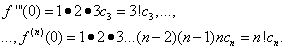
Let us show that if an arbitrary function is defined on a set  , in the vicinity of the point
  has many derivatives and is the sum of a power series:
then you can find the coefficients of this series.
Let's substitute in a power series  . Then
  .
.
Let's find the first derivative of the function  :
:
At  :
: .
.
For the second derivative we get:
At  :
: .
.
Continuing this procedure n once we get:  .
.
Thus, we obtained a power series of the form:


 ,
,
which is called next to Taylor for function  in the vicinity of the point
  .
.
A special case of the Taylor series is Maclaurin series at  :
:


The remainder of the Taylor (Maclaurin) series is obtained by discarding the main series n first members and is denoted as  . Then the function
  can be written as a sum n first members of the series
  and the remainder
  :,
:,
 .
.
The remainder is usually  expressed in different formulas.
One of them is in Lagrange form:
 , Where
  .
. .
.
Note that in practice the Maclaurin series is more often used. Thus, in order to write the function  in the form of a power series sum it is necessary:
1) find the coefficients of the Maclaurin (Taylor) series;
2) find the region of convergence of the resulting power series;
3) prove that this series converges to the function  .
.
Theorem1
(a necessary and sufficient condition for the convergence of the Maclaurin series). Let the radius of convergence of the series  . In order for this series to converge in the interval
  to function
  ,it is necessary and sufficient for the condition to be satisfied:
  in the specified interval.
Theorem 2. If derivatives of any order of the function  in some interval
  limited in absolute value to the same number M, that is
  , then in this interval the function
  can be expanded into a Maclaurin series.
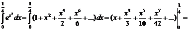
Example1
.
Expand in a Taylor series around the point  function.
Solution.
 .
.
 ,;
,;
 ,
, ;
;
 ,
, ;
;
 ,
,
.......................................................................................................................................
 ,
, ;
;
Convergence region  .
.
Example2
.
Expand a function  in a Taylor series around a point
  .
.
Solution:
Find the value of the function and its derivatives at  .
.
 ,
, ;
;
 ,
, ;
;
...........……………………………
 ,
, .
.
Let's put these values in a row. We get:
or  .
.
Let us find the region of convergence of this series. According to d'Alembert's test, a series converges if
 .
.
Therefore, for any  this limit is less than 1, and therefore the range of convergence of the series will be:
  .
.
Let us consider several examples of the Maclaurin series expansion of basic elementary functions. Recall that the Maclaurin series:


 .
.
converges on the interval  to function
  .
.
Note that to expand a function into a series it is necessary:
a) find the coefficients of the Maclaurin series for this function;
b) calculate the radius of convergence for the resulting series;
c) prove that the resulting series converges to the function  .
.
Example 3. Consider the function  .
.
Solution.
Let us calculate the value of the function and its derivatives at  .
.
Then the numerical coefficients of the series have the form:
for anyone n. Let's substitute the found coefficients into the Maclaurin series and get: 
Let us find the radius of convergence of the resulting series, namely:
 .
.
Therefore, the series converges on the interval  .
.
This series converges to the function  for any values
  , because on any interval
  function
  and its absolute value derivatives are limited in number
  .
.
Example4
.
Consider the function  .
.
Solution.
 :
:

It is easy to see that derivatives of even order  , and the derivatives are of odd order. Let us substitute the found coefficients into the Maclaurin series and obtain the expansion:
Let us find the interval of convergence of this series. According to d'Alembert's sign:
for anyone  . Therefore, the series converges on the interval
  .
.
This series converges to the function  , because all its derivatives are limited to unity.
Example5
.
 .
.
Solution.
Let us find the value of the function and its derivatives at  :
:

Thus, the coefficients of this series:  And
And  , hence:
Similar to the previous row, the area of convergence  . The series converges to the function
  , because all its derivatives are limited to unity.
Please note that the function  odd and series expansion in odd powers, function
  – even and expansion into a series in even powers.
Example6
.
Binomial series:  .
.
Solution.
Let us find the value of the function and its derivatives at  :
:

From this it can be seen that:

Let us substitute these coefficient values into the Maclaurin series and obtain the expansion of this function into a power series:
Let us find the radius of convergence of this series:

Therefore, the series converges on the interval  . At the limiting points at
  And
And  a series may or may not converge depending on the exponent
  .
.
The studied series converges on the interval  to function
  , that is, the sum of the series
  at
at  .
.
Example7
.
Let us expand the function in the Maclaurin series  .
.
Solution.
To expand this function into a series, we use the binomial series at  . We get:
Based on the property of power series (a power series can be integrated in the region of its convergence), we find the integral of the left and right sides of this series:
Let us find the area of convergence of this series:  ,
,
that is, the area of convergence of this series is the interval  . Let us determine the convergence of the series at the ends of the interval. At
 . This series is a harmonious series, that is, it diverges. At
  we get a number series with a common term
  .
.
The series converges according to Leibniz's criterion. Thus, the region of convergence of this series is the interval  .
.
16.2. Application of power series in approximate calculations
In approximate calculations, power series play an extremely important role. With their help, tables of trigonometric functions, tables of logarithms, tables of values of other functions have been compiled, which are used in various fields of knowledge, for example, in probability theory and mathematical statistics. In addition, the expansion of functions into a power series is useful for their theoretical study. The main issue when using power series in approximate calculations is the issue of estimating the error when replacing the sum of a series with the sum of its first n members.
Let's consider two cases:
the function is expanded into a sign-alternating series;
the function is expanded into a series of constant sign.
Calculation using alternating series
Let the function  expanded into an alternating power series. Then when calculating this function for a specific value
  we obtain a number series to which we can apply the Leibniz criterion. In accordance with this criterion, if the sum of a series is replaced by the sum of its first n terms, then the absolute error does not exceed the first term of the remainder of this series, that is:
  .
.
Example8
.
Calculate  with an accuracy of 0.0001.
Solution.
We will use the Maclaurin series for  , substituting the angle value in radians:

If we compare the first and second terms of the series with a given accuracy, then: .
Third term of expansion:
less than the specified calculation accuracy. Therefore, to calculate  it is enough to leave two terms of the series, that is
 .
.
Thus  .
.
Example9
.
Calculate  with an accuracy of 0.001.
Solution.
We will use the binomial series formula. To do this, let's write  as:
as:  .
.
In this expression  ,
,

Let's compare each of the terms of the series with the accuracy that is specified. It's clear that  . Therefore, to calculate
  it is enough to leave three terms of the series.
 or
or  .
.
Calculation using positive series
Example10
.
Calculate number  with an accuracy of 0.001.
Solution.
In a row for a function  let's substitute
  . We get:

Let us estimate the error that arises when replacing the sum of a series with the sum of the first  members. Let us write down the obvious inequality:
that is 2< <3.
Используем формулу остаточного члена
ряда в форме Лагранжа:
<3.
Используем формулу остаточного члена
ряда в форме Лагранжа:
 ,
, .
.
According to the problem, you need to find n such that the following inequality holds:  or
or  .
.
It is easy to check that when n= 6: .
.
Hence,  .
.
Example11
.
Calculate  with an accuracy of 0.0001.
Solution.
Note that to calculate logarithms one could use a series for the function  , but this series converges very slowly and to achieve the given accuracy it would be necessary to take 9999 terms! Therefore, to calculate logarithms, as a rule, a series for the function is used
  , which converges on the interval
  .
.
Let's calculate  using this series. Let
  , Then
  .
.
Hence,  ,
,
In order to calculate  with a given accuracy, take the sum of the first four terms:
  .
.
Rest of the series  let's discard it. Let's estimate the error. It's obvious that
or  .
.

Thus, in the series that was used for the calculation, it was enough to take only the first four terms instead of 9999 in the series for the function  .
.
Self-diagnosis questions
1. What is a Taylor series?
2. What form did the Maclaurin series have?
3. Formulate a theorem on the expansion of a function in a Taylor series.
4. Write down the Maclaurin series expansion of the main functions.
5. Indicate the areas of convergence of the considered series.
6. How to estimate the error in approximate calculations using power series?
If the function f(x) has derivatives of all orders on a certain interval containing point a, then the Taylor formula can be applied to it:
,
Where r n– the so-called remainder term or remainder of the series, it can be estimated using the Lagrange formula:
, where the number x is between x and a.
Rules for entering functions:
If for some value X r n→0 at n→∞, then in the limit the Taylor formula becomes convergent for this value Taylor series:
,
Thus, the function f(x) can be expanded into a Taylor series at the point x under consideration if:
1) it has derivatives of all orders;
2) the constructed series converges at this point.
When a = 0 we get a series called near Maclaurin:
,
Expansion of the simplest (elementary) functions in the Maclaurin series:
Exponential functions
, R=∞
Trigonometric functions ![]() , R=∞
, R=∞ ![]() , R=∞
, R=∞
, (-π/2< x < π/2), R=π/2
The function actgx does not expand in powers of x, because ctg0=∞
Hyperbolic functions
Logarithmic functions
, -1
Binomial series
![]() .
.
Example No. 1. Expand the function into a power series f(x)= 2x.
Solution. Let us find the values of the function and its derivatives at X=0
f(x) = 2x, f( 0)
= 2 0
=1;
f"(x) = 2x ln2, f"( 0)
= 2 0
ln2= ln2;
f""(x) = 2x ln 2 2, f""( 0)
= 2 0
ln 2 2= ln 2 2;
…
f(n)(x) = 2x ln n 2, f(n)( 0)
= 2 0
ln n 2=ln n 2.
Substituting the obtained values of the derivatives into the Taylor series formula, we obtain:
The radius of convergence of this series is equal to infinity, therefore this expansion is valid for -∞<x<+∞.
Example No. 2. Write the Taylor series in powers ( X+4) for function f(x)= e x.
Solution. Finding the derivatives of the function e x and their values at the point X=-4.
f(x)= e x, f(-4)
= e -4
;
f"(x)= e x, f"(-4)
= e -4
;
f""(x)= e x, f""(-4)
= e -4
;
…
f(n)(x)= e x, f(n)( -4)
= e -4
.
Therefore, the required Taylor series of the function has the form:
This expansion is also valid for -∞<x<+∞.
Example No. 3. Expand a function f(x)=ln x in a series in powers ( X- 1),
(i.e. in the Taylor series in the vicinity of the point X=1).
Solution. Find the derivatives of this function.
f(x)=lnx , , , ,
f(1)=ln1=0, f"(1)=1, f""(1)=-1, f"""(1)=1*2,..., f (n) =(- 1) n-1 (n-1)!
Substituting these values into the formula, we obtain the desired Taylor series:
Using d'Alembert's test, you can verify that the series converges at ½x-1½<1 . Действительно,
The series converges if ½ X- 1½<1, т.е. при 0<x<2. При X=2 we obtain an alternating series that satisfies the conditions of the Leibniz criterion. When x=0 the function is not defined. Thus, the region of convergence of the Taylor series is the half-open interval (0;2].
Example No. 4. Expand the function into a power series. Example No. 5. Expand the function into a Maclaurin series. Comment
.
This method is based on the theorem on the uniqueness of the expansion of a function in a power series. The essence of this theorem is that in the neighborhood of the same point two different power series cannot be obtained that would converge to the same function, no matter how its expansion is performed. Example No. 5a. Expand the function in a Maclaurin series and indicate the region of convergence. The fraction 3/(1-3x) can be considered as the sum of an infinitely decreasing geometric progression with a denominator of 3x, if |3x|< 1. Аналогично, дробь 2/(1+2x) как сумму бесконечно убывающей геометрической прогрессии знаменателем -2x, если |-2x| < 1. В результате получим разложение в степенной ряд
Example No. 6. Expand the function into a Taylor series in the vicinity of the point x = 3. Example No. 7. Write the Taylor series in powers (x -1) of the function ln(x+2) . Example No. 8. Expand the function f(x)=sin(πx/4) into a Taylor series in the vicinity of the point x =2. Example No. 1. Calculate ln(3) to the nearest 0.01. Example No. 2. Calculate to the nearest 0.0001. Example No. 3. Calculate the integral ∫ 0 1 4 sin (x) x to within 10 -5 . Example No. 4. Calculate the integral ∫ 0 1 4 e x 2 with an accuracy of 0.001.
Solution. In expansion (1) we replace x with -x 2, we get:
, -∞
Solution. We have
Using formula (4), we can write:
substituting –x instead of x in the formula, we get:
From here we find: ln(1+x)-ln(1-x) = -
Opening the brackets, rearranging the terms of the series and bringing similar terms, we get
. This series converges in the interval (-1;1), since it is obtained from two series, each of which converges in this interval.
Formulas (1)-(5) can also be used to expand the corresponding functions into a Taylor series, i.e. for expanding functions in positive integer powers ( Ha). To do this, it is necessary to perform such identical transformations on a given function in order to obtain one of the functions (1)-(5), in which instead X costs k( Ha) m , where k is a constant number, m is a positive integer. It is often convenient to make a change of variable t=Ha and expand the resulting function with respect to t in the Maclaurin series.
Solution. First we find 1-x-6x 2 =(1-3x)(1+2x) , .
to elementary:
with convergence region |x|< 1/3.
Solution. This problem can be solved, as before, using the definition of the Taylor series, for which we need to find the derivatives of the function and their values at X=3. However, it will be easier to use the existing expansion (5):
=
The resulting series converges at or –3
Solution.
The series converges at , or -2< x < 5.
Solution. Let's make the replacement t=x-2:
Using expansion (3), in which we substitute π / 4 t in place of x, we obtain:
The resulting series converges to the given function at -∞< π / 4 t<+∞, т.е. при (-∞
, (-∞Approximate calculations using power series
Power series are widely used in approximate calculations. With their help, you can calculate the values of roots, trigonometric functions, logarithms of numbers, and definite integrals with a given accuracy. Series are also used when integrating differential equations.
Consider the expansion of a function in a power series:
In order to calculate the approximate value of a function at a given point X, belonging to the region of convergence of the indicated series, the first ones are left in its expansion n members ( n– a finite number), and the remaining terms are discarded:
To estimate the error of the obtained approximate value, it is necessary to estimate the discarded remainder rn (x) . To do this, use the following techniques:
Solution. Let's use the expansion where x=1/2 (see example 5 in the previous topic):
Let's check whether we can discard the remainder after the first three terms of the expansion; to do this, we will evaluate it using the sum of an infinitely decreasing geometric progression:
So we can discard this remainder and get
Solution. Let's use the binomial series. Since 5 3 is the cube of an integer closest to 130, it is advisable to represent the number 130 as 130 = 5 3 +5. 
since already the fourth term of the resulting alternating series satisfying the Leibniz criterion is less than the required accuracy:
, so it and the terms following it can be discarded.
Many practically necessary definite or improper integrals cannot be calculated using the Newton-Leibniz formula, because its application is associated with finding the antiderivative, which often does not have an expression in elementary functions. It also happens that finding an antiderivative is possible, but it is unnecessarily labor-intensive. However, if the integrand function is expanded into a power series, and the limits of integration belong to the interval of convergence of this series, then an approximate calculation of the integral with a predetermined accuracy is possible.
Solution. The corresponding indefinite integral cannot be expressed in elementary functions, i.e. represents a “non-permanent integral”. The Newton-Leibniz formula cannot be applied here. Let's calculate the integral approximately.
Dividing term by term the series for sin x on x, we get: 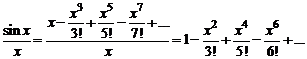
Integrating this series term by term (this is possible, since the limits of integration belong to the interval of convergence of this series), we obtain:
Since the resulting series satisfies Leibniz’s conditions and it is enough to take the sum of the first two terms to obtain the desired value with a given accuracy.
Thus, we find  .
.
Solution.
![]() . Let's check whether we can discard the remainder after the second term of the resulting series.
. Let's check whether we can discard the remainder after the second term of the resulting series.
0.0001<0.001. Следовательно, 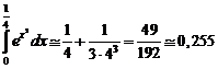 .
.