The study of a function for continuity at a point is carried out according to an already established routine scheme, which consists of checking three conditions of continuity:

Example 1

Examine the function for continuity. Determine the nature of the function discontinuities, if they exist. Execute the drawing.

Solution:

1) The only point within the scope is where the function is not defined.

One-sided limits are finite and equal.

Thus, at the point the function suffers a removable discontinuity.

What does the graph of this function look like?

I would like to simplify , and it seems like an ordinary parabola is obtained. BUT the original function is not defined at point , so the following clause is required:

Let's make the drawing:

Answer: the function is continuous on the entire number line except the point at which it suffers a removable discontinuity.

The function can be further defined in a good or not so good way, but according to the condition this is not required.

You say this is a far-fetched example? Not at all. This has happened dozens of times in practice. Almost all of the site’s tasks come from real independent work and tests.

Let's get rid of our favorite modules:

Example 2

Explore function for continuity. Determine the nature of the function discontinuities, if they exist. Execute the drawing.

Solution: For some reason, students are afraid and don’t like functions with a module, although there is nothing complicated about them. We have already touched on such things a little in the lesson. Geometric transformations of graphs. Since the module is non-negative, it is expanded as follows: , where “alpha” is some expression. IN in this case, and our function should be written piecewise:

But the fractions of both pieces must be reduced by . The reduction, as in the previous example, will not take place without consequences. The original function is not defined at the point since the denominator goes to zero. Therefore, the system should additionally specify the condition , and make the first inequality strict:

Now about the VERY USEFUL reception solutions: before finalizing the task on a draft, it is advantageous to make a drawing (regardless of whether it is required by the conditions or not). This will help, firstly, to immediately see points of continuity and points of discontinuity, and, secondly, it will 100% protect you from errors when finding one-sided limits.

Let's do the drawing. In accordance with our calculations, to the left of the point it is necessary to draw a fragment of a parabola ( Blue colour), and on the right is a piece of a parabola (red), while the function is not defined at the point itself:

If in doubt, take a few x values and plug them into the function (remembering that the module destroys the possible minus sign) and check the graph.

Let us examine the function for continuity analytically:

1) The function is not defined at the point, so we can immediately say that it is not continuous at it.

2) Let’s establish the nature of the discontinuity; to do this, we calculate one-sided limits:

The one-sided limits are finite and different, which means that the function suffers a discontinuity of the 1st kind with a jump at the point . Note that it doesn't matter whether the function at the break point is defined or not.

Now all that remains is to transfer the drawing from the draft (it was made as if with the help of research ;-)) and complete the task:

Answer: the function is continuous on the entire number line except for the point at which it suffers a discontinuity of the first kind with a jump.

Sometimes they require additional indication of the discontinuity jump. It is calculated simply - from the right limit you need to subtract the left limit: , that is, at the break point our function jumped 2 units down (as the minus sign tells us).

Example 3

Explore function for continuity. Determine the nature of the function discontinuities, if they exist. Make a drawing.

This is an example for independent decision, sample solution at the end of the lesson.

Let's move on to the most popular and widespread version of the task, when the function consists of three parts:

Example 4

Examine a function for continuity and plot a graph of the function

Solution: it is obvious that all three parts of the function are continuous on the corresponding intervals, so it remains to check only two points of “junction” between the pieces. First, let's make a draft drawing; I commented on the construction technique in sufficient detail in the first part of the article. The only thing is that we need to carefully follow our singular points: due to the inequality, the value belongs to the straight line (green dot), and due to the inequality, the value belongs to the parabola (red dot):

Well, in principle, everything is clear =) All that remains is to formalize the decision. For each of the two “joining” points, we standardly check 3 continuity conditions:

The one-sided limits are finite and different, which means that the function suffers a discontinuity of the 1st kind with a jump at the point .

Let us calculate the discontinuity jump as the difference between the right and left limits:
, that is, the graph jerked up one unit.

II) We examine the point for continuity

1) - the function is defined at a given point.

2) Find one-sided limits:

- one-sided limits are finite and equal, which means there is a general limit.

At the final stage, we transfer the drawing to the final version, after which we put the final chord:

Answer: the function is continuous on the entire number line, except for the point at which it suffers a discontinuity of the first kind with a jump.

Example 5

Examine a function for continuity and construct its graph .

This is an example for you to solve on your own, short solution and an approximate sample of the task at the end of the lesson.

You may get the impression that at one point the function must be continuous, and at another there must be a discontinuity. In practice, this is not always the case. Try not to neglect the remaining examples - there will be several interesting and important features:

Example 6

Given a function . Investigate the function for continuity at points. Build a graph.

Solution: and again immediately execute the drawing on the draft:

Peculiarity of this schedule is that when the piecewise function is given by the equation of the abscissa axis. This area is drawn here green, and in a notebook it is usually highlighted in bold with a simple pencil. And, of course, don’t forget about our rams: the value belongs to the tangent branch (red dot), and the value belongs to the straight line.

Everything is clear from the drawing - the function is continuous along the entire number line, all that remains is to formalize the solution, which is brought to full automation literally after 3-4 similar examples:

I) We examine the point for continuity

2) Let's calculate one-sided limits:

, which means there is a general limit.

A little funny thing happened here. The fact is that I created a lot of materials about the limits of a function, and several times I wanted to, but several times I forgot about one simple question. And so, with an incredible effort of will, I forced myself not to lose the thought =) Most likely, some “dummies” readers doubt: why equal limit constants? The limit of a constant is equal to the constant itself. In this case, the limit of zero is equal to zero itself (left-handed limit).

3) - the limit of a function at a point is equal to the value of this function at a given point.

Thus, a function is continuous at a point by the definition of continuity of a function at a point.

II) We examine the point for continuity

1) - the function is defined at a given point.

2) Find one-sided limits:

And here, in the right-hand limit, the limit of unity is equal to unity itself.

- there is a general limit.

3) - the limit of a function at a point is equal to the value of this function at a given point.

Thus, a function is continuous at a point by the definition of continuity of a function at a point.

As usual, after research we transfer our drawing to the final version.

Answer: the function is continuous at the points.

Please note that in the condition we were not asked anything about studying the entire function for continuity, and it is considered good mathematical form to formulate precise and clear the answer to the question posed. By the way, if the conditions do not require you to build a graph, then you have every right not to build it (although later the teacher can force you to do this).

A small mathematical “tongue twister” for solving it yourself:

Example 7

Given a function .

Investigate the function for continuity at points. Classify breakpoints, if any. Execute the drawing.

Try to “pronounce” all the “words” correctly =) And draw the graph more precisely, accuracy, it will not be superfluous everywhere;-)

As you remember, I recommended immediately completing the drawing as a draft, but from time to time you come across examples where you can’t immediately figure out what the graph looks like. Therefore, in some cases, it is advantageous to first find one-sided limits and only then, based on the study, depict the branches. In the final two examples we will also learn a technique for calculating some one-sided limits:

Example 8

Examine the function for continuity and construct its schematic graph.

Solution: the bad points are obvious: (reduces the denominator of the exponent to zero) and (reduces the denominator of the entire fraction to zero). It’s not clear what the graph of this function looks like, which means it’s better to do some research first:

I) We examine the point for continuity

2) Find one-sided limits:

pay attention to typical method for calculating a one-sided limit: instead of “x” we substitute . There is no crime in the denominator: the “addition” “minus zero” does not play a role, and the result is “four”. But in the numerator there is a little thriller going on: first we kill -1 and 1 in the denominator of the indicator, resulting in . Unit divided by , is equal to “minus infinity”, therefore: . And finally, the “two” in infinitely large negative degree equal to zero: . Or, to be even more specific: .

Let's calculate the right-hand limit:

And here - instead of “X” we substitute . In the denominator, the “additive” again does not play a role: . In the numerator, actions similar to the previous limit are carried out: we destroy opposite numbers and divide one by :

The right-hand limit is infinite, which means that the function suffers a discontinuity of the 2nd kind at the point .

II) We examine the point for continuity

1) The function is not defined at this point.

2) Let's calculate the left-sided limit:

The method is the same: we substitute “X” into the function. There is nothing interesting in the numerator - it turns out to be a finite positive number. And in the denominator we open the brackets, remove the “threes”, and decisive role"additive" plays.

As a result, the final positive number divided by infinitesimal positive number, gives “plus infinity”: .

The right-hand limit is like a twin brother, with the only exception that it appears in the denominator infinitesimal negative number:

One-sided limits are infinite, which means that the function suffers a discontinuity of the 2nd kind at the point .

Thus, we have two break points, and, obviously, three branches of the graph. For each branch, it is advisable to carry out a point-by-point construction, i.e. take several “x” values and substitute them into . Note that the condition allows the construction of a schematic drawing, and such relaxation is natural for self made. I build graphs using a program, so I don’t have such difficulties, here’s a fairly accurate picture:

Direct are vertical asymptotes for the graph of this function.

Answer: the function is continuous on the entire number line except for points at which it suffers discontinuities of the 2nd kind.

A simpler function to solve on your own:

Example 9

Examine the function for continuity and make a schematic drawing.

An approximate example of a solution at the end that crept up unnoticed.

See you soon!

Solutions and answers:

Example 3:Solution : transform the function: . Considering the modulus disclosure rule and the fact that , we rewrite the function in piecewise form:

Let's examine the function for continuity.

1) The function is not defined at the point .

The one-sided limits are finite and different, which means that the function suffers a discontinuity of the 1st kind with a jump at the point . Let's make the drawing:

Answer: the function is continuous on the entire number line except the point , in which it suffers a discontinuity of the first kind with a jump. Jump Gap: (two units up).

Example 5:Solution : Each of the three parts of the function is continuous on its own interval.
I)
1)

2) Let's calculate one-sided limits:

, which means there is a general limit.
3) - the limit of a function at a point is equal to the value of this function at a given point.
So the function continuous at a point by defining the continuity of a function at a point.
II) We examine the point for continuity

1) - the function is defined at a given point. the function suffers a discontinuity of the 2nd kind at the point

How to find the domain of a function?

Examples of solutions

If something is missing somewhere, it means there is something somewhere

We continue to study the “Functions and Graphs” section, and the next station on our journey is Function Domain. Active discussion this concept started in the first lesson about function graphs, where I looked at elementary functions, and, in particular, their domains of definition. Therefore, I recommend that dummies start with the basics of the topic, since I will not dwell on some basic points again.

It is assumed that the reader knows the domains of definition of the basic functions: linear, quadratic, cubic functions, polynomials, exponential, logarithm, sine, cosine. They are defined on . For tangents, arcsines, so be it, I forgive you =) Rarer graphs are not immediately remembered.

The scope of definition seems to be a simple thing, and a logical question arises: what will the article be about? In this lesson I will look at common problems of finding the domain of a function. Moreover, we will repeat inequalities with one variable, the solution skills of which will also be required in other problems of higher mathematics. The material, by the way, is all school material, so it will be useful not only for students, but also for students. The information, of course, does not pretend to be encyclopedic, but here are not far-fetched “dead” examples, but roasted chestnuts, which are taken from real practical works.

Let's start with a quick dive into the topic. Briefly about the main thing: we are talking about a function of one variable. Its domain of definition is many meanings of "x", for which exist meanings of "players". Let's look at a hypothetical example:

The domain of definition of this function is a union of intervals:
(for those who forgot: - unification icon). In other words, if you take any value of “x” from the interval , or from , or from , then for each such “x” there will be a value “y”.

Roughly speaking, where the domain of definition is, there is a graph of the function. But the half-interval and the “tse” point are not included in the definition area, so there is no graph there.

Yes, by the way, if anything is not clear from the terminology and/or content of the first paragraphs, it is better to return to the article Graphs and properties of elementary functions.

4.1. Basic theoretical information

Definition. Function y =f(x) called continuous at a point X 0 , if this function is defined in some neighborhood of the point X 0 and if

that is, an infinitesimal increment of the argument in the vicinity of the point X 0 corresponds to an infinitesimal increment of the function .

Definition. Function y=f(x) is continuous at the point X 0 , if it is defined in some neighborhood of this point and if the limit of the function as the independent variable tends X To X 0 exists and is equal to the value of the function at x=x 0 , that is

Definition. Let X→ X 0 , remaining all the time to the left of X 0 . If under this condition f(x) tends to the limit, then it is called the left limit of the function f(x) at the point X 0 , that is

The right limit is defined similarly

Definition. The function is continuous at the point X 0 If:

function defined at point X 0 ;

there are left and right limits of a function f(x) at X→ X 0 ;

all three numbers (X 0 ), f(x 0 –0), f(x 0 +0) coincide, that is

Definition. A function is called continuous on an interval if it is continuous at each point.

Theorem . If two functions f(x) And g(x) are defined in the same

interval and both are continuous at the point X 0 , then at the same point the functions will also be continuous

Theorem. A complex function consisting of a finite number of continuous functions is continuous.

All basic elementary functions are continuous in their domain of definition .

Definition. If at any point X 0 the function is not continuous, then the point X 0 is called the discontinuity point of the function, and the function itself is discontinuous at this point .

Definition. If at the point X 0 there is a finite lim f(x)= A

(left-hand and right-hand limits exist, are finite and equal to each other), but it does not coincide with the value of the function at the point, or the function at the point is not defined, then the point X 0 called the removable discontinuity point . Accepted point image repairable gap is shown in Fig. 1 .

Definition. A point of discontinuity of the first kind or a point of finite discontinuity is such a point X 0 , in which the function has left and right finite limits, but they are not equal to each other.

In Fig. Figure 2 shows a graphical representation of the discontinuity of a function of the first kind at the point X 0

Definition. If at least one of the limits f(x 0 – 0) or f(x 0 + 0) does not exist or is infinite, then point X 0 is called a discontinuity point of the second kind.

Graphic representations of discontinuities of functions of the second kind at a point X 0 are shown in Fig. 3 (a B C).

The above definitions of continuity of a function f(x) at point X 0

are presented in Fig. 4, where it is noted that the main premise when determining the continuity of a function (a necessary condition) at the point X 0 is that f(x) defined at a point and its surroundings .

Example: Examine for continuity, determine the nature of discontinuity points,

depict the function in the vicinity of discontinuity points

This is a rational function. It is defined and continuous for all values. X, except X= 1, since when x = 1 denominator goes to zero . IN point x = 1 function suffers a break. Let us calculate the limit of this function at

X→ 1, we have

The final limit of the function at X→ 1 exists, and the function is at the point

x = 1 not defined; means point X= 1 is a removable discontinuity point.

If we further define the function, that is, we put f (1) = 5, then the function

will be continuous.

x = 1 is shown in Fig. 4.

Comment. This function

uncertain at x = 1, coincides with a continuous function

at all points except X=1

Examine a function for continuity and determine the nature of its discontinuity points

The domain of the function is the entire number line. On the intervals (–, 0), (0,+) the function is continuous . Breaking is possible only at the point X= 0, in which the analytical specification of the function changes.

Let's find one-sided limits of the function :

The left and right limits, although finite, are not equal to each other. Therefore at the point X= 0 the function has a discontinuity of the first kind. The jump of the function at the discontinuity point is equal to

Behavior of a function in a neighborhood of a point x = 0 is shown in Fig. 5.

Rice. 5

Example Explore function f(x) for continuity, determine the nature of its discontinuity points, and depict its behavior in the vicinity of the discontinuity points.

The function is defined and continuous on the entire number line, except for points X, = –2 and X 2 = 2, and

does not exist .

Calculate one-sided limits at a point X, = –2.

So, at the point x = – 2 function suffers a discontinuity of the second kind. Let us study the nature of the discontinuity of the function at the point X 2 = 2. We have

At the point X 2 = 2 the function also suffers a discontinuity of the second kind.

Behavior of the function in the vicinity of points X X = – 2 And X 2 = 2 pictured in Fig. 6 .

Explore function f(x) = e x + i for continuity , determine the nature of the discontinuity points, depict the behavior of the function in the vicinity of the discontinuity points.

Function undefined at X= –3, so the function
continuous for all
except X= –3. Let us determine the nature of the discontinuity of the function. We have

that is, one of the limits is equal to infinity, which means the function suffers a discontinuity

second kind .

Function behavior f(x) = e x +3 in the vicinity of the break point x =–3 is shown in Fig. 7

4.2. Exercises for independent work of students

1. Examine functions for continuity, determine the nature of their discontinuity points, graphically depict the behavior of functions in the neighborhood

2. Examine functions for continuity, determine the nature of their discontinuity points, graphically depict the behavior of functions in the vicinity of discontinuity points

Continuity of function. Breaking points.

The bull walks, sways, sighs as he goes:
- Oh, the board is running out, now I’m going to fall!

In this lesson we will examine the concept of continuity of a function, the classification of discontinuity points and a common practical problem continuity studies of functions. From the very name of the topic, many intuitively guess what will be discussed and think that the material is quite simple. This is true. But it is simple tasks that are most often punished for neglect and a superficial approach to solving them. Therefore, I recommend that you study the article very carefully and catch all the subtleties and techniques.

What do you need to know and be able to do? Not very much. To learn the lesson well, you need to understand what it is limit of a function. For readers with a low level of preparation, it is enough to comprehend the article Function limits. Examples of solutions and look at the geometric meaning of the limit in the manual Graphs and properties of elementary functions. It is also advisable to familiarize yourself with geometric transformations of graphs, since practice in most cases involves constructing a drawing. The prospects are optimistic for everyone, and even a full kettle will be able to cope with the task on its own in the next hour or two!

Continuity of function. Breakpoints and their classification

Concept of continuity of function

Let's consider some function that is continuous on the entire number line:

Or, to put it more succinctly, our function is continuous on (the set real numbers).

What is the “philistine” criterion of continuity? Obviously, the graph of a continuous function can be drawn without lifting the pencil from the paper.

In this case, two simple concepts should be clearly distinguished: domain of a function And continuity of function. In general it's not the same thing. For example:

This function is defined on the entire number line, that is, for everyone The meaning of “x” has its own meaning of “y”. In particular, if , then . Note that the other point is punctuated, because by the definition of a function, the value of the argument must correspond to the only thing function value. Thus, domain our function: .

However this function is not continuous on ! It is quite obvious that at the point she is suffering gap. The term is also quite intelligible and visual; indeed, here the pencil will have to be torn off the paper anyway. A little later we will look at the classification of breakpoints.

Continuity of a function at a point and on an interval

In a particular mathematical problem, we can talk about the continuity of a function at a point, the continuity of a function on an interval, a half-interval, or the continuity of a function on a segment. That is, there is no “mere continuity”– the function can be continuous SOMEWHERE. And the fundamental “building block” of everything else is continuity of function at the point .

The theory of mathematical analysis gives a definition of the continuity of a function at a point using “delta” and “epsilon” neighborhoods, but in practice there is a different definition in use, to which we will pay close attention.

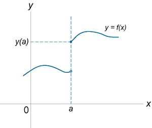
First let's remember one-sided limits who burst into our lives in the first lesson about function graphs. Consider an everyday situation:

If we approach the axis to the point left(red arrow), then the corresponding values of the “games” will go along the axis to the point (crimson arrow). Mathematically, this fact is fixed using left-hand limit:

Pay attention to the entry (reads “x tends to ka on the left”). The “additive” “minus zero” symbolizes , essentially this means that we are approaching the number from the left side.

Similarly, if you approach the point “ka” on right(blue arrow), then the “games” will come to the same value, but along the green arrow, and right-hand limit will be formatted as follows:

"Additive" symbolizes , and the entry reads: “x tends to ka on the right.”

If one-sided limits are finite and equal(as in our case): , then we will say that there is a GENERAL limit. It's simple, the general limit is our “usual” limit of a function, equal to a finite number.

Note that if the function is not defined at (puncture black dot on the graph branch), then the above calculations remain valid. As has already been noted several times, in particular in the article on infinitesimal functions, expressions mean that "x" infinitely close approaches the point, while DOESN'T MATTER, whether the function itself is defined at a given point or not. Good example will appear in the next paragraph, when the function is analyzed.

Definition: a function is continuous at a point if the limit of the function at a given point is equal to the value of the function at that point: .

The definition is detailed in following conditions:

1) The function must be defined at the point, that is, the value must exist.

2) There must be a general limit of the function. As noted above, this implies the existence and equality of one-sided limits: .

3) The limit of the function at a given point must be equal to the value of the function at this point: .

If violated at least one of the three conditions, then the function loses the property of continuity at the point .

Continuity of a function over an interval is formulated ingeniously and very simply: a function is continuous on the interval if it is continuous at every point of the given interval.

In particular, many functions are continuous on an infinite interval, that is, on the set of real numbers. This is a linear function, polynomials, exponential, sine, cosine, etc. And in general, any elementary function continuous on its domain of definition, for example, a logarithmic function is continuous on the interval . Hopefully by now you have a pretty good idea of what graphs of basic functions look like. More detailed information their continuity can be gleaned from kind person by the surname Fichtengolts.

With the continuity of a function on a segment and half-intervals, everything is also not difficult, but it is more appropriate to talk about this in class about finding the minimum and maximum values of a function on a segment, but for now let’s not worry about it.

Classification of break points

The fascinating life of functions is rich in all sorts of special points, and break points are only one of the pages of their biography.

Note : just in case, I’ll dwell on an elementary point: the breaking point is always single point– there are no “several break points in a row”, that is, there is no such thing as a “break interval”.

These points, in turn, are divided into two large groups: ruptures of the first kind And ruptures of the second kind. Each type of gap has its own characteristics which we will look at right now:

Discontinuity point of the first kind

If the continuity condition is violated at a point and one-sided limits finite , then it is called discontinuity point of the first kind.

Let's start with the most optimistic case. According to the original idea of the lesson, I wanted to tell the theory “in general view”, but in order to demonstrate the reality of the material, I settled on the option with specific characters.

It’s sad, like a photo of newlyweds against the backdrop of the Eternal Flame, but the following shot is generally accepted. Let us depict the graph of the function in the drawing:

This function is continuous on the entire number line, except for the point. And in fact, the denominator cannot be equal to zero. However, in accordance with the meaning of the limit, we can infinitely close approach “zero” both from the left and from the right, that is, one-sided limits exist and, obviously, coincide:
(Condition No. 2 of continuity is satisfied).

But the function is not defined at the point, therefore, Condition No. 1 of continuity is violated, and the function suffers a discontinuity at this point.

A break of this type (with the existing general limit) are called repairable gap. Why removable? Because the function can redefine at the breaking point:

Does it look weird? Maybe. But such a function notation does not contradict anything! Now the gap is closed and everyone is happy:

Let's perform a formal check:

2) – there is a general limit;
3)

Thus, all three conditions are satisfied, and the function is continuous at a point by the definition of continuity of a function at a point.

However, matan haters can define the function in a bad way, for example :

It is interesting that the first two continuity conditions are satisfied here:
1) – the function is defined at a given point;
2) – there is a general limit.

But the third boundary has not been passed: , that is, the limit of the function at the point not equal the value of a given function at a given point.

Thus, at a point the function suffers a discontinuity.

The second, sadder case is called rupture of the first kind with a jump. And sadness is evoked by one-sided limits that finite and different. An example is shown in the second drawing of the lesson. Such a gap usually occurs when piecewise defined functions, which have already been mentioned in the article about graph transformations.

Consider the piecewise function and we will complete its drawing. How to build a graph? Very simple. On a half-interval we draw a fragment of a parabola ( green color), on the interval – a straight line segment (red) and on a half-interval – a straight line (blue).

Moreover, due to inequality, the value is determined for quadratic function(green dot), and due to the inequality , the value is defined for the linear function (blue dot):

In the most difficult case, you should resort to point-by-point construction of each piece of the graph (see the first lesson about graphs of functions).

Now we will only be interested in the point. Let's examine it for continuity:

2) Let's calculate one-sided limits.

On the left we have a red line segment, so the left-sided limit is:

On the right is the blue straight line, and the right-hand limit:

As a result, we received finite numbers, and they not equal. Since one-sided limits finite and different: , then our function tolerates discontinuity of the first kind with a jump.

It is logical that the gap cannot be eliminated - the function really cannot be further defined and “glued together”, as in the previous example.

Discontinuity points of the second kind

Usually, all other cases of rupture are cleverly classified into this category. I won’t list everything, because in practice, in 99% of problems you will encounter endless gap– when left-handed or right-handed, and more often, both limits are infinite.

And, of course, the most obvious picture is the hyperbola at point zero. Here both one-sided limits are infinite: , therefore, the function suffers a discontinuity of the second kind at the point .

I try to fill my articles with as diverse content as possible, so let's look at the graph of a function that has not yet been encountered:

according to the standard scheme:

1) The function is not defined at this point because the denominator goes to zero.

Of course, we can immediately conclude that the function suffers a discontinuity at point , but it would be good to classify the nature of the discontinuity, which is often required by the condition. For this:

Let me remind you that by recording we mean infinitesimal negative number, and under the entry - infinitesimal positive number.

One-sided limits are infinite, which means that the function suffers a discontinuity of the 2nd kind at the point . The y-axis is vertical asymptote for the graph.

It is not uncommon for both one-sided limits to exist, but only one of them is infinite, for example:

This is the graph of the function.

We examine the point for continuity:

1) The function is not defined at this point.

2) Let's calculate one-sided limits:

We will talk about the method of calculating such one-sided limits in the last two examples of the lecture, although many readers have already seen and guessed everything.

The left-hand limit is finite and equal to zero (we “do not go to the point itself”), but the right-hand limit is infinite and the orange branch of the graph approaches infinitely close to its vertical asymptote, given by the equation (black dotted line).

So the function suffers second kind discontinuity at point .

As for a discontinuity of the 1st kind, the function can be defined at the discontinuity point itself. For example, for a piecewise function Feel free to put a black bold dot at the origin of coordinates. On the right is a branch of a hyperbola, and the right-hand limit is infinite. I think almost everyone has an idea of what this graph looks like.

What everyone was looking forward to:

How to examine a function for continuity?

The study of a function for continuity at a point is carried out according to an already established routine scheme, which consists of checking three conditions of continuity:

Example 1

Explore function

Solution:

1) The only point within the scope is where the function is not defined.

2) Let's calculate one-sided limits:

One-sided limits are finite and equal.

Thus, at the point the function suffers a removable discontinuity.

What does the graph of this function look like?

I would like to simplify , and it seems like an ordinary parabola is obtained. BUT the original function is not defined at point , so the following clause is required:

Let's make the drawing:

Answer: the function is continuous on the entire number line except the point at which it suffers a removable discontinuity.

The function can be further defined in a good or not so good way, but according to the condition this is not required.

You say this is a far-fetched example? Not at all. This has happened dozens of times in practice. Almost all of the site’s tasks come from real independent work and tests.

Let's get rid of our favorite modules:

Example 2

Explore function for continuity. Determine the nature of the function discontinuities, if they exist. Execute the drawing.

Solution: For some reason, students are afraid and don’t like functions with a module, although there is nothing complicated about them. We have already touched on such things a little in the lesson. Geometric transformations of graphs. Since the module is non-negative, it is expanded as follows: , where “alpha” is some expression. In this case, and our function should be written piecewise:

Now about a VERY USEFUL decision technique: before finalizing the task on a draft, it is advantageous to make a drawing (regardless of whether it is required by the conditions or not). This will help, firstly, to immediately see points of continuity and points of discontinuity, and, secondly, it will 100% protect you from errors when finding one-sided limits.

Let's do the drawing. In accordance with our calculations, to the left of the point it is necessary to draw a fragment of a parabola (blue color), and to the right - a piece of a parabola (red color), while the function is not defined at the point itself:

If in doubt, take a few x values and plug them into the function (remembering that the module destroys the possible minus sign) and check the graph.

Let us examine the function for continuity analytically:

1) The function is not defined at the point, so we can immediately say that it is not continuous at it.

2) Let’s establish the nature of the discontinuity; to do this, we calculate one-sided limits:

The one-sided limits are finite and different, which means that the function suffers a discontinuity of the 1st kind with a jump at the point . Note again that when finding limits, it does not matter whether the function at the break point is defined or not.

Now all that remains is to transfer the drawing from the draft (it was made as if with the help of research ;-)) and complete the task:

Answer: the function is continuous on the entire number line except for the point at which it suffers a discontinuity of the first kind with a jump.

Example 3

Explore function for continuity. Determine the nature of the function discontinuities, if they exist. Make a drawing.

This is an example for you to solve on your own, a sample solution at the end of the lesson.

Let's move on to the most popular and widespread version of the task, when the function consists of three parts:

Example 4

Examine a function for continuity and plot a graph of the function .

I) We examine the point for continuity

The one-sided limits are finite and different, which means that the function suffers a discontinuity of the 1st kind with a jump at the point .

Let us calculate the discontinuity jump as the difference between the right and left limits:
, that is, the graph jerked up one unit.

II) We examine the point for continuity

1) – the function is defined at a given point.

2) Find one-sided limits:

– one-sided limits are finite and equal, which means there is a general limit.

3) – the limit of a function at a point is equal to the value of this function at a given point.

At the final stage, we transfer the drawing to the final version, after which we put the final chord:

Answer: the function is continuous on the entire number line, except for the point at which it suffers a discontinuity of the first kind with a jump.

Example 5

Examine a function for continuity and construct its graph .

This is an example for independent solution, a short solution and an approximate sample of the problem at the end of the lesson.

Example 6

Given a function . Investigate the function for continuity at points. Build a graph.

Solution: and again immediately execute the drawing on the draft:

The peculiarity of this graph is that the piecewise function is given by the equation of the abscissa axis. Here this area is drawn in green, but in a notebook it is usually highlighted in bold with a simple pencil. And, of course, don’t forget about our rams: the value belongs to the tangent branch (red dot), and the value belongs to the straight line.

I) We examine the point for continuity

1) – the function is defined at a given point.

2) Let's calculate one-sided limits:

, which means there is a general limit.

Just in case, let me remind you of a trivial fact: the limit of a constant is equal to the constant itself. In this case, the limit of zero is equal to zero itself (left-handed limit).

3) – the limit of a function at a point is equal to the value of this function at a given point.

Thus, a function is continuous at a point by the definition of continuity of a function at a point.

II) We examine the point for continuity

1) – the function is defined at a given point.

2) Find one-sided limits:

And here – the limit of one is equal to the unit itself.

– there is a general limit.

3) – the limit of a function at a point is equal to the value of this function at a given point.

Thus, a function is continuous at a point by the definition of continuity of a function at a point.

As usual, after research we transfer our drawing to the final version.

Answer: the function is continuous at the points.

A small mathematical “tongue twister” for solving it yourself:

Example 7

Given a function . Investigate the function for continuity at points. Classify breakpoints, if any. Execute the drawing.

Try to “pronounce” all the “words” correctly =) And draw the graph more precisely, accuracy, it will not be superfluous everywhere;-)

Example 8

Examine the function for continuity and construct its schematic graph.

Solution: the bad points are obvious: (reduces the denominator of the exponent to zero) and (reduces the denominator of the entire fraction to zero). It is not clear what the graph of this function looks like, which means it is better to do some research first.

Definition function break points and their types is a continuation of the theme of continuity of function. A visual (graphical) explanation of the meaning of break points of a function is also given in contrast with the concept of continuity. Let's learn how to find breakpoints of a function and determine their types. And our faithful friends will help us with this - the left and right limits, generally called one-sided limits. If anyone has any fear of unilateral limits, we will soon dispel it.

Points on a graph that are not connected to each other are called function break points . The graph of such a function, which suffers a discontinuity at the point x=2 - - in the figure below.

A generalization of the above is the following definition. If a function is not continuous at a point, then it has a discontinuity at this point and the point itself is called break point . Disruptions are of the first kind and of the second kind .

In order to determine types (character) of break points functions need to be found with confidence limits, so it’s a good idea to open the corresponding lesson in a new window. But in connection with breakpoints, we have something new and important - one-sided (left and right) limits. In general they are written (right limit) and (left limit). As in the case of a limit in general, in order to find the limit of a function, you need to substitute X in the expression of the function for what X tends to. But, perhaps, you ask, how will the right and left limits differ, if in the case of the right one something is added to X, but this something is zero, and in the case of the left one something is subtracted from X, but this something - also zero? And you'll be right. In most cases.

But in the practice of searching for discontinuity points of a function and determining their type, there are two typical cases when the right and left limits are not equal:

a function has two or more expressions depending on the portion of the number line to which x belongs (these expressions are usually written in curly brackets after f(x)= );
as a result of substituting what X tends to, we get a fraction in the denominator of which remains either plus zero (+0) or minus zero (-0) and therefore such a fraction means either plus infinity or minus infinity, and these are completely different things.

Discontinuity points of the first kind

Break point of the first kind: a function has both a finite (i.e., not equal to infinity) left limit and a finite right limit, but the function is not defined at a point or the left and right limits are different (not equal).

Point of removable discontinuity of the first kind. The left and right limits are equal. In this case, it is possible to further define the function at a point. To define a function at a point, simply speaking, means to provide a connection of points between which there is a point at which the left and right limits are found equal to each other. In this case, the connection should represent only one point at which the value of the function should be found.

Example 1. Determine the break point of the function and the type (character) of the break point.

Discontinuity points of the second kind

Break point of the second kind: the point at which at least one of the limits (left or right) is infinite (equal to infinity).

Example 3.

Solution. From the expression for the power at e it is clear that the function is not defined at the point. Let's find the left and right limits of the function at this point:

One of the limits is equal to infinity, so the point is a discontinuity point of the second kind. The graph of a function with a break point is below the example.

Finding breakpoints of a function can be either an independent task or part of Full function research and graphing .

Example 4. Determine the break point of the function and the type (character) of the break point for the function

Solution. From the expression for the power at 2 it is clear that the function is not defined at the point. Let's find the left and right limits of the function at this point.

If the function f(x) is not continuous at the point x = a, then they say that f(x) It has gap at this point. Figure 1 schematically shows the graphs of four functions, two of which are continuous at x = a, and two have a gap.


Continuous at x = a.		Has a gap at x = a.

Continuous at x = a.		Has a gap at x = a.
Picture 1.

Classification of function discontinuity points

All breakpoints of the function are divided into discontinuity points of the first and second kind .

They say the function f(x) It has discontinuity point of the first kind at x = a, if at this point

In this case, the following two cases are possible:

Function f(x) It has point of discontinuity of the second kind at x = a, if at least one of the one-sided limits does not exist or is equal to infinity.

Example3.13 Consider the function (Heaviside function) on the segment,. Then it is continuous on the segment (despite the fact that at the point it has a discontinuity of the first kind).

Fig. 3.15 Graph of the Heaviside function

A similar definition can be given for half-intervals, including cases. However, we can generalize this definition for the case of an arbitrary subset as follows. Let us first introduce the concept of an induced base: let be a base all of whose endings have non-empty intersections with. Let us denote by and consider the set of all. It is then easy to check that the set will be the base. Thus, bases are defined for, and, where, and are the bases of unpunctured two-sided (left, right, respectively) neighborhoods of a point (see their definition at the beginning of the current chapter).

Properties of functions continuous on an interval.

Property 1: (Weierstrass's first theorem (Carl Weierstrass (1815-1897) - German mathematician)). A function that is continuous on an interval is bounded on this interval, i.e. on the segment [ a, b ] the condition is fulfilled - M £ f (x) £ M.

The proof of this property is based on the fact that a function that is continuous at the point x 0 is bounded in some neighborhood of it, and if we split the segment [ a, b ] into an infinite number of segments that are “contracted” to the point x 0, then a certain neighborhood of the point x 0 is formed.

Property 2: A function continuous on the interval [ a, b ], takes the largest and smallest values on it.

Those. there are values of x 1 and x 2 such that f (x 1 ) = m , f (x 2 ) = M , and

m £ f (x) £ M

Let us note these largest and smallest values; the function can take on a segment several times (for example - f(x) = sinx).

The difference between the largest and smallest value of a function on a segment is called hesitation functions on a segment.

Property 3: (Second Bolzano-Cauchy theorem). A function continuous on the interval [ a, b ], takes on this segment all values between two arbitrary values.

Property 4: If the function f(x ) is continuous at the point x = x 0, then there is a certain neighborhood of the point x 0 in which the function retains its sign.

Property 5: (First theorem of Bolzano (1781-1848) - Cauchy). If the function f(x ) - continuous on the segment [ a, b ] and has values of opposite signs at the ends of the segment, then there is a point inside this segment where f(x) = 0.

T . e. If sign(f(a))¹ sign(f(b)), then $ x 0 : f(x 0) = 0.

Definition. Function f(x ) is called uniformly continuous on the segment [ a, b ], if for any e >0 exists D >0 such that for any points x 1О [ a , b ] and x 2 О [ a , b ] such that

ï x 2 - x 1 ï< D

inequality trueï f (x 2 ) - f (x 1 ) ï< e

The difference between uniform continuity and “ordinary” continuity is that for any e exists its own D , independent of x, and with “ordinary” continuity D depends on e and x.

Property 6: Cantor's theorem (Georg Cantor (1845-1918) - German mathematician). A function continuous on a segment is uniformly continuous on it.

(This property is true only for segments, and not for intervals and half-intervals.)

Example .