Page 21 of 37
Classification of a company's costs in the short term.
When analyzing costs, it is necessary to distinguish costs for the entire output, i.e. general (full, total) production costs, and production costs per unit of production, i.e. average (unit) costs.
Considering the costs of the entire output, one can find that when the volume of production changes, the value of some types of costs does not change, while the value of other types of costs is variable.
Fixed costs (F.C. – fixed costs) are costs that do not depend on the volume of production. These include the costs of maintaining buildings, major renovation, administrative and management expenses, rent, property insurance payments, some types of taxes.
The concept of fixed costs can be illustrated in Fig. 5.1. Let us plot the quantity of products produced on the x-axis (Q), and on the ordinate - costs (WITH). Then the fixed cost schedule (FC) will be a straight line parallel to the x-axis. Even when the enterprise does not produce anything, the value of these costs is not zero.
Rice. 5.1. Fixed costs
Variable costs(V.C. – variable costs) are costs, the value of which varies depending on changes in production volumes. Variable costs include costs of raw materials, materials, electricity, workers' compensation, expenses for auxiliary materials.
Variable costs increase or decrease in proportion to output (Fig. 5.2). On initial stages produced

Rice. 5.2. Variable costs
production, they grow at a faster rate than manufactured products, but as optimal output is reached (at the point Q 1) the growth rate of variable costs is decreasing. In larger firms, unit costs per unit of output are lower due to increased production efficiency, which is ensured by more high level specialization of workers and more complete use of capital equipment, so the growth of variable costs becomes slower than the increase in output. In the future, when the enterprise exceeds its optimal size, the law of diminishing returns (profitability) comes into play and variable costs are again beginning to outpace production growth.
Law of Diminishing Marginal Productivity (Profitability) states that, starting from a certain point in time, each additional unit of a variable factor of production brings a smaller increase in total output than the previous one. This law takes place when any factor of production remains unchanged, for example, production technology or the size of the production territory, and is valid only for a short period of time, and not over a long period of human existence.
Let us explain the operation of the law using an example. Let's assume that the enterprise has a fixed amount of equipment and workers work in one shift. If an entrepreneur hires additional workers, work can be carried out in two shifts, which will lead to an increase in productivity and profitability. If the number of workers increases further, and workers begin to work in three shifts, then productivity and profitability will increase again. But if you continue to hire workers, there will be no increase in productivity. Such a constant factor as equipment has already exhausted its capabilities. The addition of additional variable resources (labor) to it will no longer give the same effect; on the contrary, starting from this moment, the costs per unit of output will increase.
The law of diminishing marginal productivity underlies the behavior of the profit-maximizing producer and determines the nature of the supply function on price (the supply curve).
It is important for an entrepreneur to know to what extent he can increase production volume so that variable costs do not become very large and do not exceed the profit margin. The differences between fixed and variable costs are significant. A manufacturer can control variable costs by changing the volume of output. Fixed costs must be paid regardless of production volume and are therefore beyond the control of management.
General costs(TS– total costs) is a set of fixed and variable costs of the company:
TC= F.C. + V.C..
Total costs are obtained by summing the fixed and variable cost curves. They repeat the configuration of the curve V.C., but are spaced from the origin by the amount F.C.(Fig. 5.3).

Rice. 5.3. General costs
For economic analysis, average costs are of particular interest.
Average costs is the cost per unit of production. The role of average costs in economic analysis determined by the fact that, as a rule, the price of a product (service) is set per unit of production (per piece, kilogram, meter, etc.). Comparing average costs with price allows you to determine the amount of profit (or loss) per unit of product and decide on the feasibility of further production. Profit serves as a criterion for choosing the right strategy and tactics for a company.
The following types of average costs are distinguished:
Average fixed costs ( AFC – average fixed costs) – fixed costs per unit of production:
АFC= F.C. / Q.
As production volume increases, fixed costs are distributed across all large quantity products, so that average fixed costs decrease (Fig. 5.4);
Average variable costs ( AVC – average variable costs) – variable costs per unit of production:
AVC= V.C./ Q.
As production volume increases AVC first they fall, due to increasing marginal productivity (profitability) they reach their minimum, and then, under the influence of the law of diminishing returns, they begin to increase. So the curve AVC has an arched shape (see Fig. 5.4);
average total costs ( ATS – average total costs) – total costs per unit of production:
ATS= TS/ Q.
Average costs can also be obtained by adding average fixed and average variable costs:
ATC= A.F.C.+ AVC.
The dynamics of average total costs reflects the dynamics of average fixed and average variable costs. While both are decreasing, average total costs are falling, but when, as production volume increases, the growth of variable costs begins to outpace the fall in fixed costs, average total costs begin to rise. Graphically, average costs are depicted by summing the curves of average fixed and average variable costs and have a U-shape (see Fig. 5.4).

Rice. 5.4. Production costs per unit of production:
MS – limit, AFC – average constants, АВС – average variables,
ATS – average total production costs
The concepts of total and average costs are not enough to analyze the behavior of a company. Therefore, economists use another type of cost - marginal.
Marginal cost(MS – marginal costs) are the costs associated with producing an additional unit of output.
The marginal cost category is of strategic importance because it allows you to show the costs that the company will have to incur if it produces one more unit of output or
save if production is reduced by this unit. In other words, marginal cost is a value that a firm can directly control.
Marginal costs are obtained as the difference between total production costs ( n+ 1) units and production costs n product units:
MS= TSn+1 – TSn or MS= D TS/D Q,
where D is a small change in something,
TS– total costs;
Q- volume of production.
Marginal costs are presented graphically in Figure 5.4.
Let us comment on the basic relationships between average and marginal costs.
1. Marginal costs ( MS) do not depend on fixed costs ( FC), since the latter do not depend on production volume, but MS- These are incremental costs.
2. While marginal costs are less than average ( MS< AC), the average cost curve has a negative slope. This means that producing an additional unit of output reduces average cost.
3. When marginal costs are equal to average ( MS = AC), this means that average costs have stopped decreasing, but have not yet begun to increase. This is the point of minimum average cost ( AC= min).
4. When marginal costs become greater than average costs ( MS> AC), the average cost curve slopes upward, indicating an increase in average costs as a result of producing an additional unit of output.
5. Curve MS intersects the average variable cost curve ( ABC) and average costs ( AC) at the points of their minimum values.
To calculate costs and estimate production activities enterprises in the West and Russia use various methods. Our economy has widely used methods based on the category production costs, which includes the total costs of production and sales of products. To calculate the cost, costs are classified into direct, directly going towards the creation of a unit of goods, and indirect, necessary for the functioning of the company as a whole.
Based on the previously introduced concepts of costs, or costs, we can introduce the concept added value, which is obtained by subtracting from total income or the revenue of a variable cost enterprise. In other words, it consists of fixed costs and net profit. This indicator is important for assessing production efficiency.
To determine the total costs of producing different volumes of output and the costs per unit of output, it is necessary to combine production data included in the law of diminishing returns with information on input prices. As already noted, during short term time some resources related to technical equipment enterprises remain unchanged. The number of other resources may vary. It follows that in the short term different kinds costs can be classified as either fixed or variable.
Fixed costs. Fixed costs are those costs whose value does not change depending on changes in production volume. Fixed costs are associated with existence itself production equipment companies and must be paid even if the company does not produce anything. Fixed costs, as a rule, include payment of obligations on bond loans, bank loans, lease payments, enterprise security, payment utilities(telephone, lighting, sewerage), as well as time-based salaries for employees of the enterprise.
Variable costs. Variables are those costs whose value changes depending on changes in production volume. These include costs of raw materials, fuel, energy, transport services, for the majority of labor resources, etc. The amount of variable costs varies depending on production volumes.
General costs is the sum of fixed and variable costs for each given volume of production.
We show total, fixed and variable costs on the graph (see Fig. 1).

At zero production volume, total costs are equal to the sum of the firm's fixed costs. Then, with the production of each additional unit of output (from 1 to 10), the total cost changes by the same amount as the sum of the variable costs.
The sum of variable costs changes from the origin, and the sum of fixed costs is added each time to the vertical dimension of the sum of variable costs to obtain the total cost curve.
The distinction between fixed and variable costs is significant. Variable costs are costs that can be quickly controlled; their value can be changed over a short period of time by changing production volume. On the other hand, fixed costs are obviously beyond the control of the firm's management. Such costs are mandatory and must be paid regardless of production volumes.
Allows you to calculate the minimum price of goods/services, determine the optimal volume of sales and calculate the value of the company's expenses. There are various methods of calculating by type of costs, the main ones are given below.
Production costs - calculation formulas
Calculation of production costs is easily carried out on the basis of estimate documentation. If such forms are not drawn up in the organization, data from the reporting period of accounting will be required. It should be taken into account that all costs are divided into fixed (the value remains unchanged over the period) and variable (the value changes depending on production volumes).
Total production costs - formula:
Total costs = Fixed costs + Variable costs.
This calculation method allows you to find out the total costs for the entire production. Detailing is carried out by departments of the enterprise, workshops, product groups, types of products, etc. Analysis of indicators over time will help predict the volume of production or sales, expected profit/loss, the need to increase capacity, and the inevitability of reducing expenditures.
Average production costs - formula:
Average costs = Total costs / Volume of manufactured products/performed services.
This indicator is also called the total cost of the product/service. Allows you to determine the level minimum price, calculate the efficiency of investing resources for each unit of production, compare mandatory costs with prices.
Marginal cost of production - formula:
Marginal costs = Change in total costs / Change in production volume.
The indicator of so-called additional costs makes it possible to determine the increase in costs for the production of additional volume of GP in the most profitable way. At the same time, the amount of fixed costs remains unchanged, while variable costs increase.
Note! In accounting, an enterprise's expenses are reflected in cost accounts - 20, 23, 26, 25, 29, 21, 28. To determine costs for the required period, you should sum up the debit turnover on the accounts involved. Internal turnover and balances at refineries are subject to exclusion.
How to calculate production costs - example
|
Volume of production of GP, pcs. |
Total costs, rub. |
Average costs, rub. |
Fixed costs, rub. |
Variable costs, rub. |
From the above example it is clear that the organization incurs fixed costs in the amount of 1200 rubles. in any case - in the presence or absence of production of goods. Variable expenses for 1 piece initially amount to 150 rubles, but costs are reduced as production increases. This can be seen from the analysis of the second indicator - Average costs, which decreased from 1350 rubles. up to 117 rub. per 1 unit of finished product. Calculation of marginal costs can be determined by dividing the increase in variable costs by 1 unit of product or by 5, 50, 100, etc.
Economic and accounting costs.
In economics costs most often referred to as losses that a manufacturer (entrepreneur, firm) is forced to bear in connection with the implementation of economic activities. This could be: the cost of money and time for organizing production and acquiring resources, loss of income or product from missed opportunities; costs of collecting information, concluding contracts, promoting goods to the market, preserving goods, etc. When choosing among different resources and technologies, a rational manufacturer strives for minimum costs, therefore selects the most productive and cheapest resources.
The production costs of any product can be represented as a set of physical or cost units of resources expended in its production. If we express the value of all these resources in monetary units ah, then we get the cost expression of the costs of producing this product. This approach will not be wrong, but it seems to leave unanswered the question of how the value of these resources will be determined for the subject, which will determine this or that line of his behavior. The economist's task is to choose the best option for using resources.
Costs in the economy are directly related to the denial of the possibility of producing alternative goods and services. This means that the cost of any resource equals its cost, or value, given the best of all possible options its use.
It is necessary to distinguish between external and internal costs.
External or explicit costs– these are cash expenses for paying for resources owned by other companies (payment for raw materials, fuel, wage and etc.). These costs, as a rule, are taken into account by an accountant, reflected in the financial statements and are therefore called accounting.
At the same time, the company can use its own resources. In this case, costs are also inevitable.
Internal costs – These are the costs of using the firm's own resources that do not take the form of cash payments.
These costs are equal to the cash payments that the firm could receive for its own resources if it chose the best option for using them.
Economists consider all external and internal payments as costs, including the latter and normal profit.
Normal, or zero, profit - this is the minimum fee necessary to maintain the entrepreneur's interest in the chosen activity. This is the minimum payment for the risk of working in a given area of the economy, and in each industry it is assessed differently. It is called normal for its similarity to other incomes, reflecting the contribution of a resource to production. Zero - because in essence it is not a profit, representing a part of the total production costs.
Example. You are the owner of a small store. You purchased goods worth 100 million rubles. If accounting costs for the month amounted to 500 thousand rubles, then to them you must add lost rent (let’s say 200 thousand rubles), lost interest (let’s say you could put 100 million rubles in the bank at 10% per annum, and receive approximately 900 thousand rubles) and a minimum risk fee (let’s say it is equal to 600 thousand rubles). Then the economic costs will be
500 + 200 + 900 + 600 = 2200 thousand rubles.
Production costs in the short term, their dynamics.
The production costs that a firm incurs in producing products depend on the possibility of changing the amount of all employed resources. Some types of costs can be changed quite quickly ( work force, fuel, etc.), others require a certain time for this.
Based on this, short-term and long-term periods are distinguished.
Short term – This is the period of time during which a firm can change production volume only due to variable costs, while production capacity remains unchanged. For example, hire additional workers, purchase more raw materials, use equipment more intensively, etc. It follows that in the short run costs can be either constant or variable.
Fixed costs (F.C.) - These are costs whose value does not depend on the volume of production.
Fixed costs are associated with the very existence of the firm and must be paid even if the firm does not produce anything. These include: rental payments, deductions for depreciation of buildings and equipment, insurance premiums, interest on loans, and labor costs for management personnel.
Variable costs (V.C.) - These are costs, the value of which changes depending on changes in production volume.
With zero output they are absent. These include: costs of raw materials, fuel, energy, most labor resources, transport services, etc. The firm can control these costs by changing production volume.
Total production costs (TC) – This is the sum of fixed and variable costs for the entire volume of output.
TC = total fixed costs (TFC) + total variable costs (TVC).
There are also average and marginal costs.
Average costs – This is the cost per unit of production. Average short-term costs are divided into average fixed, average variable and average total.
Average fixed costs (A.F.C.) are calculated by dividing total fixed costs by the number of products produced.
Average variable costs (AVC) are calculated by dividing total variable costs by the number of products produced.
Average Total Cost (ATC) are calculated using the formula
ATS = TS / Q or ATS = AFC + AVC
To understand the behavior of a firm, the category of marginal costs is very important.
Marginal cost (MC)– These are additional costs associated with producing one more unit of output. They can be calculated using the formula:
MS =∆ TC / ∆ Qwhere ∆Q= 1
In other words, marginal cost is the partial derivative of the total cost function.
Marginal costs make it possible for a firm to determine whether it is advisable to increase production of goods. To do this, compare marginal costs with marginal revenue. If marginal costs are less than the marginal revenue received from sales of this unit of product, then production can be expanded.
As production volumes change, costs change. Graphical representation of cost curves reveals some important patterns.

Fixed costs, given their independence from production volumes, do not change.
Variable costs are zero when there is no output; they increase as output increases. Moreover, at first the growth rate of variable costs is high, then it slows down, but upon reaching a certain level of production, it increases again. This nature of the dynamics of variable costs is explained by the laws of increasing and diminishing returns.
Gross costs are equal to fixed costs when output is zero, and as production increases, the gross cost curve follows the shape of the variable cost curve.

Average fixed costs will continuously decrease following the growth of production volumes. This is because fixed costs are spread over more units of production.
The average variable cost curve is U-shaped.
The average total cost curve also has this shape, which is explained by the relationship between the dynamics of AVC and AFC.
The dynamics of marginal costs are also determined by the law of increasing and diminishing returns.
The MC curve intersects the AVC and AC curves at the points of the minimum value of each of them. This dependence of the limit and average values has a mathematical basis.
Types of tasks:
· Tasks on deriving formulas for all types of costs used in economic theory;
· Problems on the relationship between total, average, marginal costs;
· Tasks for calculating sales revenue;
· Tasks for calculating depreciation charges.
· Tasks to determine the effect of scale of production.
4.1 . Let's say the total costs of a firm to produce Q units of output are: TC = 2Q² + 10Q + 162.
A) Derive functions of all types of costs used in economic theory to describe the behavior of a company;
B) At what values of Q does average total cost reach its minimum?
Solution:
· FC=162, fixed costs;
· VC = 2Q² + 10Q, variable costs;
· A.F.C.=FC/Q= 162/Q, average fixed costs;
· AVC=VC/Q= 2Q+10, average variable costs;
· ATC= TC / Q = (FC / Q + VC / Q) = ( 2Q + 10) + 162/Q, average total costs;
· M.C.=dTC/dQ= 4Q+10, marginal costs.
B) The minimum average total cost occurs at the intersection of the ATC and MC schedules, therefore, we equate these functions:
2Q + 10 + 162 / Q = 4Q + 10;
2Q² + 10Q + 162 = 4Q² + 10Q;
Min ATC achieved upon release (Q) = 9; at given volume production has reached production optimum.
4.2. The total cost function is:
TC = 36 + 12Q + Q². Determine what the average fixed costs are for a production volume of 10.
Solution:
AFC = FC / Q where FC = 36, because fixed costs do not depend on the volume of products produced.
Therefore: AFC = 36/10 = 3.6.
Answer: 3,6.
4.3. Determine the maximum revenue if demand up to the intersection with the axes is described by a linear function: Q(D) = b – aР, where P is the price of the goods produced by the entrepreneur; b and a are the coefficients of the demand function.
Solution:
First option:
a) According to economic theory, an entrepreneur achieves maximum revenue (income) when selling a product:
· at a price equal to half the prohibitive price (A/2);
· with a sales volume equal to half the saturation mass (B/2) (see Fig. 4.5).
The formula for maximum revenue is as follows:
TR max = A/2 × B/2.
b) Find the values of the prohibitive price and saturation mass:
· at Q(D) = 0, the price value P = A = b/a (the value of the prohibitive price);
· at P = 0 the value of Q(D) = B = b (saturation mass value).
Rice. 4.5. Graph of linear demand function Q(D) = b – a Р.
· A/2 = (b/a):2 = b/2a;
d) Hence the value of the maximum revenue will be:
TR = b/2a × b/2 = b²/4a.
Second option:
According to the conditions of the problem, the quantity of demand is: Q(D) = b – aP. Let us determine the price at which the entrepreneur receives maximum revenue: TR = P × Q = P × (b – aP).
a) To do this, we equate the price derivative of the revenue function to zero: (P × (b – aP))’ = 0. We get the price: P = b / 2a.
b) Determine the volume of production at which the entrepreneur will receive maximum revenue. Let's substitute the price value into the demand function: Q(D) = b – a × b / 2a = b / 2; ==> Q(D) = b / 2.
c) Therefore, the maximum revenue of the entrepreneur will be: TRmax = Q × P = b / 2 × b / 2a = b² / 4a.
Answer: b²/4a.
4.4. The firm's output under conditions perfect competition–1000 units products, product price - 80 USD, total average costs (ATC) for the production of 1000 units. goods - 30. Determine the amount of accounting profit.
Solution:
a) we calculate accounting profit using the formula: PR = TR – TC. Then company revenue will be TR= 80 × 1000 = 80 000 .
b) Using the average total cost formula:
· calculate the value of total costs using the formula: AC = TC / Q and
· let's express total costs: 30 = TC / 1000; TC = 30,000.
c) Then profit PR = 80 000 – 30 000 = 50 000
Answer: 50 000.
4.5 . A truck worth 100 thousand rubles. It will take 250 thousand km before it is written off. What is the amount of depreciation?
Solution:
Depreciation- this is a reduction in the accounting value of capital resources and the gradual transfer of their value to the cost of the manufactured product as they wear out.
There are various methods of calculating depreciation:
straightforward method
· accelerated method,
· service unit method.
We will use the service unit method because physical standard wear and tear is associated with the provision of services. Consequently, depreciation charges per 1 km will be 0.4 rubles. regardless of service life.
Answer: 0.4 rub. for 1 km.
4.6. Demand functions are given Q(D) = 220 – 4Р and marginal costs MC = 10 + 4Q. Maximum profit is 125 monetary units. Determine the amount of fixed costs.
Solution:
To determine the value of fixed costs, we derive the equation for the total cost function: TC = FC + V.C.. To do this, we find the antiderivative of the marginal cost function MC = 10 + 4Q. The equation for the total cost function will take the form: TC = 10Q + 2Q² + FC.
1. Let us determine the volume of production that maximizes profit by applying the profit maximization rule MC = MR.
2. Let us derive the equation of the function marginal income. If we apply the marginal revenue formula: MR = (TR)" = (P × Q)", then we get that MR = ((55 – 0.25Q) × Q)"(where P = 55 – 0.25Q is inverse function for the demand function Q(D) = 220 – 4Р). Hence, the equation of the marginal income function will be as follows: MR = 55 – 0.5Q. Therefore, the production volume Qopt, which maximizes profit, will be 10 units.
3. Let's calculate the value of total revenue TR(Qopt 10) = 55Q – 0.25Q² = 525.
4. Let's find the value of total costs using the profit formula:
PR = TR – TC,
PR = 125, and TR = 525. Amount of total costs TC will be 400.
Let us equate the equation of the total cost function with the value of total costs: 400 = 10Q + 2Q²+FC, where Qopt= 10.
Hence, FC= 100.